Page 53 - Geochemical Anomaly and Mineral Prospectivity Mapping in GIS

52 Chapter 3

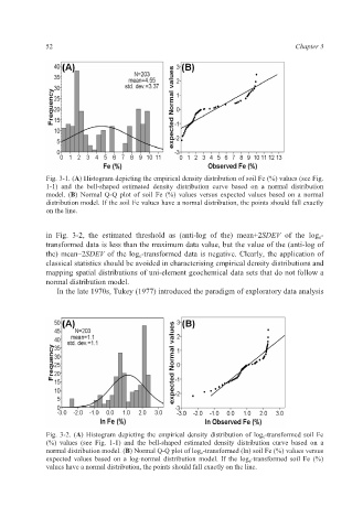
Fig. 3-1. (A) Histogram depicting the empirical density distribution of soil Fe (%) values (see Fig.
1-1) and the bell-shaped estimated density distribution curve based on a normal distribution
model. (B) Normal Q-Q plot of soil Fe (%) values versus expected values based on a normal
distribution model. If the soil Fe values have a normal distribution, the points should fall exactly
on the line.

in Fig. 3-2, the estimated threshold as (anti-log of the) mean+2SDEV of the log e-
transformed data is less than the maximum data value, but the value of the (anti-log of
the) mean–2SDEV of the log e-transformed data is negative. Clearly, the application of
classical statistics should be avoided in characterising empirical density distributions and
mapping spatial distributions of uni-element geochemical data sets that do not follow a
normal distribution model.
In the late 1970s, Tukey (1977) introduced the paradigm of exploratory data analysis

Fig. 3-2. (A) Histogram depicting the empirical density distribution of log e -transformed soil Fe
(%) values (see Fig. 1-1) and the bell-shaped estimated density distribution curve based on a
normal distribution model. (B) Normal Q-Q plot of log e -transformed (ln) soil Fe (%) values versus
expected values based on a log-normal distribution model. If the log e -transformed soil Fe (%)
values have a normal distribution, the points should fall exactly on the line.