Page 58 - Geochemical Anomaly and Mineral Prospectivity Mapping in GIS

Exploratory Analysis of Geochemical Anomalies 57

Classification of uni-element geochemical data
Based on a boxplot, an exploration uni-element geochemical data set can usually be
divided into five robust classes (Fig. 3-4): (1) minimum–LW; (2) LW–LH; (3) LH–UH;
(4) UH–UW; and (5) UW–maximum. The UIF is usually considered the threshold
separating background values and anomalies (e.g., Bounessah and Atkin, 2003; Reimann
et al., 2005), although the UOF can also be used as the threshold (e.g., Yusta et al.,
1998). However, an estimated value representing the UIF (equation (3.4)) may not be
actually part of an exploration uni-element geochemical data set, so that outliers beyond
the UW represent anomalies. Thus, data values in the UH–UW class (at most 25% of a
data set) can be considered high background, data values in the LH–UH class (at most
50% of a data set) are background, data values in the LW–LH class (at most 25% of a
data set) are low background and data values in the minimum–LW class are extremely
low background.
Aside from the boxplot-defined threshold (e.g., UIF or UW), a threshold can be
defined from the EDA statistics as median+2MAD. The MAD is the median absolute
deviation, which is estimated as the median of absolute deviations of all data values from
the data median (Tukey, 1977):

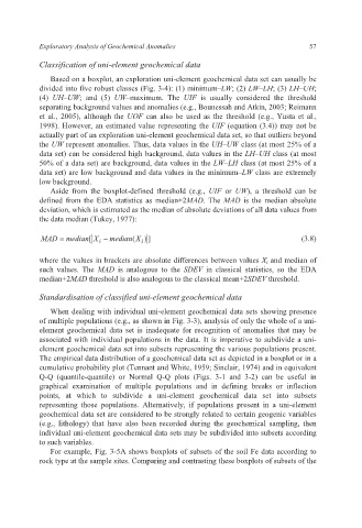
MAD = median [ X − median (X i ] ) (3.8)
i

where the values in brackets are absolute differences between values X i and median of
such values. The MAD is analogous to the SDEV in classical statistics, so the EDA
median+2MAD threshold is also analogous to the classical mean+2SDEV threshold.

Standardisation of classified uni-element geochemical data
When dealing with individual uni-element geochemical data sets showing presence
of multiple populations (e.g., as shown in Fig. 3-3), analysis of only the whole of a uni-
element geochemical data set is inadequate for recognition of anomalies that may be
associated with individual populations in the data. It is imperative to subdivide a uni-
element geochemical data set into subsets representing the various populations present.
The empirical data distribution of a geochemical data set as depicted in a boxplot or in a
cumulative probability plot (Tennant and White, 1959; Sinclair, 1974) and in equivalent
Q-Q (quantile-quantile) or Normal Q-Q plots (Figs. 3-1 and 3-2) can be useful in
graphical examination of multiple populations and in defining breaks or inflection
points, at which to subdivide a uni-element geochemical data set into subsets
representing those populations. Alternatively, if populations present in a uni-element
geochemical data set are considered to be strongly related to certain geogenic variables
(e.g., lithology) that have also been recorded during the geochemical sampling, then
individual uni-element geochemical data sets may be subdivided into subsets according
to such variables.
For example, Fig. 3-5A shows boxplots of subsets of the soil Fe data according to
rock type at the sample sites. Comparing and contrasting these boxplots of subsets of the