Page 59 - Geochemical Anomaly and Mineral Prospectivity Mapping in GIS

58 Chapter 3

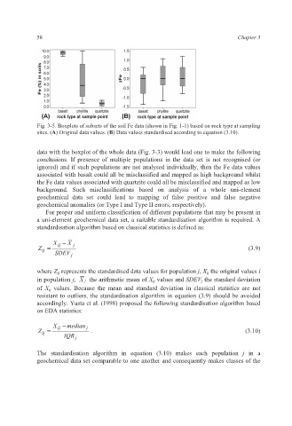
Fig. 3-5. Boxplots of subsets of the soil Fe data (shown in Fig. 1-1) based on rock type at sampling
sites. (A) Original data values. (B) Data values standardised according to equation (3.10).

data with the boxplot of the whole data (Fig. 3-3) would lead one to make the following
conclusions. If presence of multiple populations in the data set is not recognised (or
ignored) and if such populations are not analysed individually, then the Fe data values
associated with basalt could all be misclassified and mapped as high background whilst
the Fe data values associated with quartzite could all be misclassified and mapped as low
background. Such misclassifications based on analysis of a whole uni-element
geochemical data set could lead to mapping of false positive and false negative
geochemical anomalies (or Type I and Type II errors, respectively).
For proper and uniform classification of different populations that may be present in
a uni-element geochemical data set, a suitable standardisation algorithm is required. A
standardisation algorithm based on classical statistics is defined as:

X − X
Z = ij j (3.9)
ij
SDEV j

where Z ij represents the standardised data values for population j, X ij the original values i
in population j, X the arithmetic mean of X ij values and SDEV j the standard deviation
j
of X ij values. Because the mean and standard deviation in classical statistics are not
resistant to outliers, the standardisation algorithm in equation (3.9) should be avoided
accordingly. Yusta et al. (1998) proposed the following standardisation algorithm based
on EDA statistics:

X − median
Z = ij j . (3.10)
ij
IQR j

The standardisation algorithm in equation (3.10) makes each population j in a
geochemical data set comparable to one another and consequently makes classes of the