Page 214 - Geometric Modeling and Algebraic Geometry

12 Approximate Implicitization of Space Curves and of Surfaces of Revolution 217
where w 1 and w 2 are positive weights satisfying 1 >w 1 >>w 2 > 0. The first
weight controls the influence of the estimated normal vectors n i to the resulting
curve. As observed in our experiments, increasing the weights w 1 or w 2 can be
used to ‘push away’ unwanted branches of the curve from the region of interest.
The tension term T in (12.2) is added in order to control the shape of the result-
ing curve. It pulls the approximating curve towards a simpler shape. A possible
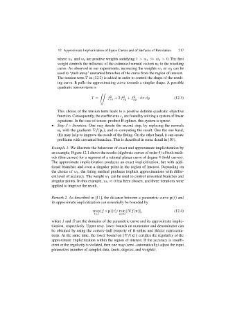
quadratic tension term is
--
T = f 2 +2 f 2 + f 2 dx dy (12.3)
xx xy yy
Ω

This choice of the tension term leads to a positive definite quadratic objective
function. Consequently, the coefficients c j are found by solving a system of linear
equations. In the case of tensor–product B-splines, this system is sparse.
• Step 3 – Iteration: One may iterate the second step, by replacing the normals
n i with the gradients ∇f(p i ), and re–computing the result. One the one hand,
this may help to improve the result of the fitting. On the other hand, it can create
problems with unwanted branches. This is described in some detail in [10].
Example 1. We illustrate the behaviour of exact and approximate implicitization by
an example. Figure 12.1 shows the results (algebraic curves of order 4) of both meth-
ods (thin curves) for a segment of a rational planar curve of degree 4 (bold curves).
The approximate implicitization produces an exact implicitization, but with addi-
tional branches and even a singular point in the region of interest. Depending on
the choice of w 1 , the fitting method produces implicit approximations with differ-
ent level of accuracy. The weight w 1 can be used to control unwanted branches and
singular points. In this example, w 2 ≈ 0 has been chosen, and three iterations were
applied to improve the result.

Remark 2. As described in [11], the distance between a parametric curve p(t) and
its approximate implicitization can essentially be bounded by

max(f ◦ p)(t)/ min &∇f(x)&, (12.4)
t∈I x∈Ω
where I and Ω are the domains of the parametric curve and its approximate implic-
tization, respectively. Upper resp. lower bounds on numerator and denominator can
be obtained by using the convex–hull property of B-spline and B´ ezier representa-
tions. At the same time, the lower bound on &∇f(x)& certifies the regularity of the
approximate implicitization within the region of interest. If the accuracy is insuffi-
cient or the regularity is violated, then one may (semi–automatically) adjust the input
parameters (number of sampled data, knots, degrees, and weights).