Page 215 - Geometric Modeling and Algebraic Geometry

218 M. Shalaby and B. J¨uttler

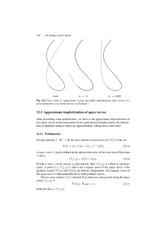
exact w 1 =1.0 w 1 =0.0001
Fig. 12.1. Exact (left) vs. approximate (center and right) implicitization (thin curves) of a
given parametric curve (bold curves), see Example 1.

12.3 Approximate implicitization of space curves

After presenting some preliminaries, we discuss the approximate implicitization of
two space curves as the intersection of two generalized cylinders and as the intersec-
tion of algebraic surfaces which are approximately orthogonal to each other.

12.3.1 Preliminaries

For any function f : R → R, the zero contour (or zero level set) Z(f) is the set
3
Z(f)= {x | f(x)=0} = f −1 ({0}) (12.5)

A space curve C can be defined as the intersection curve of two zero sets of functions
f and g,
C(f, g)= Z(f) ∩Z(g). (12.6)
If both f and g can be chosen as polynomials, then C(f, g) is called an algebraic
curve. A point x ∈ C(f, g) is said to be a regular point of the space curve, if the
gradient vectors ∇f(x) and ∇g(x) are linearly independent. The tangent vector of
the space curve is then perpendicular to both gradient vectors.
The two zero contours Z(f) and and Z(g) intersect orthogonally along the space
curve C(f, g),if
∇f(x) ·∇g(x)=0 (12.7)
holds for all x ∈ C(f, g).