Page 220 - Geometric Modeling and Algebraic Geometry

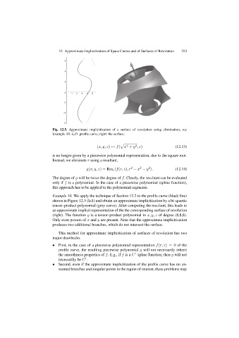
12 Approximate Implicitization of Space Curves and of Surfaces of Revolution 223

6

4

2

0
1 2 3 4 5
–2

–4

–6
Fig. 12.5. Approximate implicitization of a surface of revolution using elimination, see
Example 10. Left: profile curve, right: the surface.

&
(x, y, z) → f( x + y ,z) (12.13)
2
2
is no longer given by a piecewise polynomial representation, due to the square root.
Instead, we eliminate r using a resultant,
g(x, y, z)= Res r (f(r, z),r − x − y ). (12.14)
2
2
2
The degree of g will be twice the degree of f. Clearly, the resultant can be evaluated
only if f is a polynomial. In the case of a piecewise polynomial (spline function),
this approach has to be applied to the polynomial segments.
Example 10. We apply the technique of Section 12.2 to the profile curve (black line)
shown in Figure 12.5 (left) and obtain an approximate implicitization by a bi–quartic
tensor–product polynomial (grey curve). After computing the resultant, this leads to
an approximate implicit representation of the the corresponding surface of revolution
(right). The function g is a tensor–product polynomial in x, y, z of degree (8,8,8).
Only even powers of x and y are present. Note that the approximate implicitization
produces two additional branches, which do not intersect the surface.

This method for approximate implicitization of surfaces of revolution has two
major drawbacks.
• First, in the case of a piecewise polynomial representation f(r, z)=0 of the
profile curve, the resulting piecewise polynomial g will not necessarily inherit
the smoothness properties of f. E.g., if f is a C spline function, then g will not
1
necessarily be C .
1
• Second, even if the approximate implicitization of the profile curve has no un-
wanted branches and singular points in the region of interest, these problems may