Page 216 - Geometric Modeling and Algebraic Geometry

12 Approximate Implicitization of Space Curves and of Surfaces of Revolution 219

1.4 1.4
1.2 1.2
z 1 z 1
0.8 0.8
0.6 0.6
1 1
0.5 1 0.5 0.5 1 0.5
1.5
2 1.5 2
x 2.5 y x 2.5 y
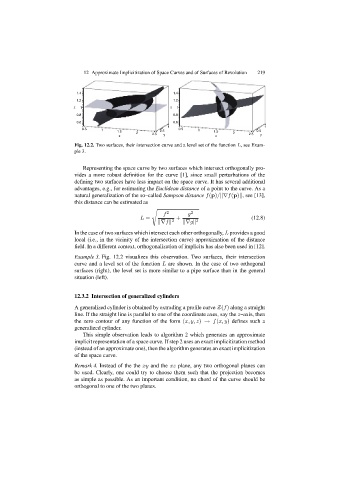
Fig. 12.2. Two surfaces, their intersection curve and a level set of the function L, see Exam-
ple 3.
Representing the space curve by two surfaces which intersect orthogonally pro-
vides a more robust definition for the curve [1], since small perturbations of the
defining two surfaces have less impact on the space curve. It has several additional
advantages, e.g., for estimating the Euclidean distance of a point to the curve. As a
natural generalization of the so–called Sampson distance f(p)/||∇f(p)||, see [13],
this distance can be estimated as
.
f 2 g 2
L = + (12.8)
&∇f& 2 &∇g& 2
In the case of two surfaces which intersect each other orthogonally, L provides a good
local (i.e., in the vicinity of the intersection curve) approximation of the distance
field. In a different context, orthogonalization of implicits has also been used in [12].
Example 3. Fig. 12.2 visualizes this observation. Two surfaces, their intersection
curve and a level set of the function L are shown. In the case of two orthogonal
surfaces (right), the level set is more similar to a pipe surface than in the general
situation (left).

12.3.2 Intersection of generalized cylinders

A generalized cylinder is obtained by extruding a profile curve Z(f) along a straight
line. If the straight line is parallel to one of the coordinate axes, say the z–axis, then
the zero contour of any function of the form (x, y, z) → f(x, y) defines such a
generalized cylinder.
This simple observation leads to algorithm 2 which generates an approximate
implicit representation of a space curve. If step 2 uses an exact implicitization method
(instead of an approximate one), then the algorithm generates an exact implicitization
of the space curve.

Remark 4. Instead of the the xy and the xz plane, any two orthogonal planes can
be used. Clearly, one could try to choose them such that the projection becomes
as simple as possible. As an important condition, no chord of the curve should be
orthogonal to one of the two planes.