Page 218 - Geometric Modeling and Algebraic Geometry

12 Approximate Implicitization of Space Curves and of Surfaces of Revolution 221
0.6 0.6
0.5 0.5
0.4 0.4
y 0.3 y 0.3
0.2 0.2
0.1 0.1
0 0.2 0.4 0.6 0.8 1 0 0.2 0.4 0.6 0.8 1
x x
=10 3 =10 −3
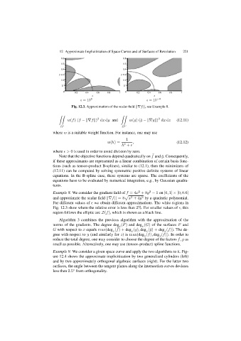
Fig. 12.3. Approximation of the scalar field ||∇f||, see Example 8.

-- --
¯
g
w(f)(f −&∇f&) dx dy and w(g)(¯ −&∇g&) dx dz (12.11)
2
2
Ω Ω
where w is a suitable weight function. For instance, one may use
1
w(h)= , (12.12)
h +
2
where > 0 is used in order to avoid division by zero.
¯
g
Note that the objective functions depend quadratically on f and ¯. Consequently,
if these approximants are represented as a linear combination of certain basis func-
tions (such as tensor–product B-splines), similar to (12.1), then the minimizers of
(12.11) can be computed by solving symmetric positive definite systems of linear
equations. In the B-spline case, these systems are sparse. The coefficients of the
equations have to be evaluated by numerical integration, e.g., by Gaussian quadra-
tures.
Example 8. We consider the gradient field of f =4x +8y − 1 on [0, 1] × [0, 0.6]
2
2
&
and approximate the scalar field ||∇f|| =8 x +4y by a quadratic polynomial.
2
2
For different values of we obtain different approximations. The white regions in
Fig. 12.3 show where the relative error is less than 2%. For smaller values of ,this
region follows the elliptic arc Z(f), which is shown as a black line.
Algorithm 3 combines the previous algorithm with the approximation of the
norms of the gradients. The degree deg (F) and deg (G) of the surfaces F and
x
x
¯
G with respect to x equals max(deg (f)+ deg (g), deg (¯g)+ deg (f)). The de-
x
x
x
x
¯
gree with respect to y (and similarly for z)is max(deg (f), deg (f)). In order to
x
x
¯
g
reduce the total degree, one may consider to choose the degree of the factors f, ¯ as
small as possible. Alternatively, one may use (tensor–product) spline functions.
Example 9. We consider a given space curve and apply the two algorithms to it. Fig-
ure 12.4 shows the approximate implicitization by two generalized cylinders (left)
and by two approximately orthogonal algebraic surfaces (right). For the latter two
surfaces, the angle between the tangent planes along the intersection curves deviates
less then 2.5 from orthogonality.
◦