Page 176 - Glucose Monitoring Devices

178 CHAPTER 9 Calibration of CGM systems

(A) (B)

FIGURE 9.4
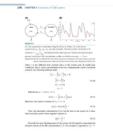
(A) Two-compartment model describing the BG-to-IG kinetics. R a is the rate of
appearance; k 01 , k 02 , k 12 , k 21 are rate constants. The time constant of the BG-to-IG
1
system is s ¼ . (B) Representative blood glucose (dashed line) and interstitial
k 02 þ k 12
glucose (continuous line) concentration profiles simulated assuming s ¼ 11 min.
Adapted from Acciaroli G, Vettoretti M, Facchinetti A, Sparacino G. Calibration of minimally invasive continuous
glucose monitoring sensors: state-of-the-art and current perspectives. Biosensors 2018;8(1):24.
where s is the diffusion time constant and a is the system gain. In steady-state
conditions, that is, when concentrations in the two compartments can be considered
constant, the following relations hold:
1

a
C I ¼ C I þ C B ¼ 0
s s
1 a
C I ¼ C B (9.10)
s s
C I ¼ a$C B
a ¼ 1
Substituting a ¼ 1in Eq. (9.9),
1 1

C I ðtÞ¼ C I ðtÞþ C B ðtÞ (9.11)
s s
Moreover, the explicit solution of Eq. (9.11) is
1 t
C I ðtÞ¼ C B ðtÞ5 e s (9.12)
s
Thus, the interstitial concentration C I ðtÞ can be seen as the output of a linear
time-invariant system whose impulse response is
1 t
hðtÞ¼ e s (9.13)
s
Given the low-pass filtering nature of the system, the IG signal is a smoothed and
delayed version of the BG concentration [22]. An example is reported in Fig. 9.4