Page 205 - Glucose Monitoring Devices

208 CHAPTER 10 CGM filtering and denoising techniques

are retrospectively tuned and are not individualized. To solve both these problems, the
2
2
following two-step procedure for the estimation of l and s can be used.
Step 1
The first portion of each CGM time series is considered as a tuning interval, where
2
2
the unknown parameters l and s are automatically estimated using a stochastically
based smoothing criterion based on maximum before (ML). The tuning interval
should contain a suitable number of CGM values, for example, some tens (hereafter
we will call this number N). Briefly, approaching the problem of smoothing the data
of the tuning interval in vector y ¼ [y(1) y(2) . y(N)] as a linear minimum variance
estimation problem, and also defining u ¼ [u(1) u(2) . u(N)] and v ¼ [v(1) v(2) .
v(N)], one has to solve:

2
T T
T
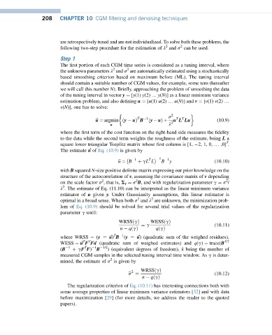
b u ¼ argmin ðy uÞ B 1 ðy uÞþ s u L Lu (10.9)
u l 2
where the first term of the cost function on the right-hand side measures the fidelity
to the data while the second term weights the roughness of the estimate, being L a
T
square lower triangular Toeplitz matrix whose first column is [1, 2, 1, 0, . ,0] .
The estimate u ˆ of Eq. (10.9) is given by
1 T 1 1
b u ¼ B þ gL L B y (10.10)
with B squared N-size positive definite matrix expressing our prior knowledge on the
structure of the autocorrelation of v, assuming the covariance matrix of v depending
2
2
2
on the scale factor s , that is, S v ¼ s B, and with regularization parameter g ¼ s /
2
l . The estimate of Eq. (11.10) can be interpreted as the linear minimum variance
estimator of u given y. Under Gaussianity assumptions, this linear estimator is
2
2
optimal in a broad sense. When both s and l are unknown, the minimization prob-
lem of Eq. (10.9) should be solved for several trial values of the regularization
parameter g until:
WRSSðgÞ WESSðgÞ
(10.11)
¼ g
n qðgÞ qðgÞ
T
1
where WRSS ¼ (y L u ˆ) B (y L u ˆ) (quadratic sum of the weighed residues),
T
T
WESS ¼ u ˆ F Fu ˆ (quadratic sum of weighed estimates) and q(g) ¼ trace(B 1/2
T
1 1/2
(B 1 þ gF F) B ) (equivalent degrees of freedom), k being the number of
measured CGM samples in the selected tuning interval time window. As g is deter-
2
mined, the estimate of s is given by
2 WRSSðgÞ
b s ¼ (10.12)
n qðgÞ
The regularization criterion of Eq. (10.11) has interesting connections both with
some average properties of linear minimum variance estimators [32] and with data
before maximization [29] (for more details, we address the reader to the quoted
papers).