Page 239 - Glucose Monitoring Devices

Methods 243

spaced, reference SMBG data points. After elimination of missing data
segments and nonfunctioning sensors, the final dataset was composed of 20,660
reference/sensor data pairs.
2. The second dataset is smaller but more controlled, in that BG was measured
every 15 min in clinical settings, using YSI instruments (coefficient of var-
iation ¼ 2%). It contains navigator sensor readings taken every minute in 28
patients, two sensors per patient at different sites, that is, 56 sensors. After
elimination of missing data and nonfunctioning sensors, the final dataset was
composed of approximately 7000 data pairs.

A posteriori recalibration
Ae previously mentioned, CGMs yield estimates that are the product of (at least)
two consecutive steps: (1) deduction of BG values from IG-related electrical
current recorded by the sensor and (2) blood-to-interstitial glucose transport. To
assess the impact of calibration errors (i.e., step (1)), we performed a posteriori
recalibration of the data foreachsensorleveragingthe method generally used
by sensor producers, that is, linear/quadratic fitting with time-delay compensation.
The major difference between a posteriori and real-time calibration is the availabil-
ity of all reference BG points; therefore, for a fixed calibration function (the rela-
tion between sensor current and BG), a posteriori calibration is optimal in
minimizing the sensor readings-reference glucose discrepancy. In this study, a
posteriori calibration was performed by linear regression, matching the interpo-
lated sensor readings (if the timing of the reference fell between two readings of
the sensor) to the reference measurements. The sum of squares was assessed
only at the points of reference measurement. The result of the linear regression
was considered to be the recalibrated sensor trace.

Reference-sensor density and delay estimation
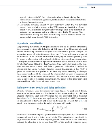
Density estimation. Once the sensors were recalibrated, we used kernel density
estimation to approximate the distribution of the sensor readings for different
glucose references. Each sensor/reference pair was associated with a Gaussian
kernel (see Eq. 12.1) centered on the pair and of predetermined width. More details
on the selection of the width and kernel function can be found in Ref. [18]. The
density was then computed as the weighted sum of all kernels:
N 2 2
1 X ððs s iÞ þðr r iÞ Þ
Dðs; rÞ¼ 2 e 2s 2 (12.1)
2ps N
i¼1
where N is the number of pairs, s i is the sensor reading of pair i, r i is the reference
measure of pair i,and s is the kernel width. This estimation of the density is
slightly biased by the fact that negative glucose values do not occur; the bias is
reducedbychoosing s to be less than 25% of the smallest reference value.