Page 496 - Handbook of Electrical Engineering

486 HANDBOOK OF ELECTRICAL ENGINEERING

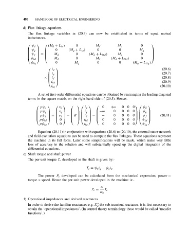
d) Flux linkage equations
The flux linkage variables in (20.5) can now be established in terms of equal mutual
inductances.

   0 0 
ψ d (M d + L la ) M d M d
0 (M q + L la ) 0 0
 ψ q   M q 
   0 0 
M d (M d + L lf d ) M d
 ψ f  =  
   0 (M d + L lkd ) 0 
ψ kd M d M d
0 0 0 (M q + L lkq )
ψ kq M q
 
i d (20.6)
(20.7)
 i q 
(20.8)
 
×  i f 
 
i kd (20.9)
i kq (20.10)
A set of first-order differential equations can be obtained by rearranging the leading diagonal
terms in the square matrix on the right-hand side of (20.5). Hence:-
           
pψ d v d i d 0 +ω 0 0 0 ψ d
 −ω 0 0
 pψ q   v q     i q  0 0   ψ q 
           
 pψ f  =  v f  −  R   i f  −  − 0 0 0 0   ψ f  (20.11)
   0       0 0 0 0 0   
pψ kd i kd ψ kd
0 0 0 0 0 0
pψ kq i kq ψ kq
Equation (20.11) in conjunction with equations (20.6) to (20.10), the external stator network
and field excitation equations can be used to compute the flux linkages. These equations represent
the machine in its full form. Later some simplifications will be made, which make very little
loss of accuracy in the solution and will substantially speed up the digital integration of the
differential equations.
e) Shaft torque and shaft power
The per-unit torque T e developed in the shaft is given by:-

T e = ψ d i q − ψ q i d

The power P e developed can be calculated from the mechanical expression, power =
torque × speed. Hence the per-unit power developed in the machine is:-
ω
P e = T e
ω n
f) Operational impedances and derived reactances

In order to derive the familiar reactances e.g. X the sub-transient reactance, it is first necessary to
d
obtain the ‘operational impedances’. (In control theory terminology these would be called ‘transfer
functions’.)