Page 497 - Handbook of Electrical Engineering

GENERALISED THEORY OF ELECTRICAL MACHINES 487

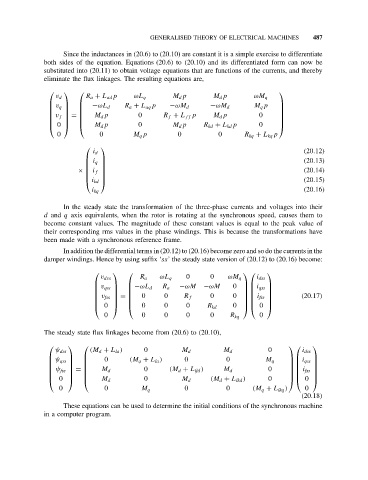
Since the inductances in (20.6) to (20.10) are constant it is a simple exercise to differentiate
both sides of the equation. Equations (20.6) to (20.10) and its differentiated form can now be
substituted into (20.11) to obtain voltage equations that are functions of the currents, and thereby
eliminate the flux linkages. The resulting equations are,

   
R a + L ad p M d p M d p
v d ωL q ωM q
   R a + L aq p M q p 
−ωL d −ωM d −ωM d
 v q   
M d p 0 R f + L ff p M d p 0
   
 v f  =  
   
M d p 0 M d p R kd + L kd p 0
 0   
0 0 M q p 0 0 R kq + L kq p
 
i d (20.12)
 i  (20.13)
 q 
(20.14)
 
×  i f 
 
 i kd  (20.15)
(20.16)
i kq
In the steady state the transformation of the three-phase currents and voltages into their
d and q axis equivalents, when the rotor is rotating at the synchronous speed, causes them to
become constant values. The magnitude of these constant values is equal to the peak value of
their corresponding rms values in the phase windings. This is because the transformations have
been made with a synchronous reference frame.
In addition the differential terms in (20.12) to (20.16) become zero and so do the currents in the
damper windings. Hence by using suffix ‘ss’ the steady state version of (20.12) to (20.16) become:

     
v dss R a ωL q 0 0 ωM q i dss
v −ωL d R a −ωM −ωM 0 i
     
 qss     qss 
0 0 0 (20.17)
     
 v fss  =  R f 0   i fss 
     
0 0 0
 0   R kd 0   0 
0 0 0 0 0 R kq 0
The steady state flux linkages become from (20.6) to (20.10),
     
(M d + L la ) 0 0
ψ dss M d M d i dss
0 (M q + L la ) 0 0 M q i
     
 ψ qss     qss 
     
M d 0 (M d + L lfd ) M d 0
 ψ fss  =    i fss 
     
 0   M d 0 M d (M d + L lkd ) 0   0 
0 0 M q 0 0 (M q + L lkq ) 0
(20.18)
These equations can be used to determine the initial conditions of the synchronous machine
in a computer program.