Page 206 - Handbook of Materials Failure Analysis

202 CHAPTER 8 Seismic risk of RC water storage elevated tanks

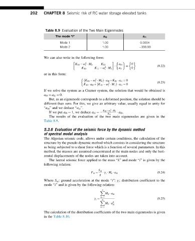
Table 8.9 Evaluation of the Two Main Eigenmodes
The mode “i” a i0 a i1
Mode 1 1.00 0.0004
Mode 2 1.00 399.99

We can also write in the following form:

2

K 00 ω M 0 K 01 a i0 0
i (8.22)
2 ¼
K 10 K 11 ω M 1 a i1 0
i
or in this form:
2
K 00 ω M 0 a i0 + K 01 a i1 ¼ 0

i
2
K 10 a i0 + K 11 ω M 1 a i1 ¼ 0 (8.23)
i
If we solve the system as a Cramer system, the solution that would be obtained is
a i0 ¼ a i1 ¼ 0.
But, as an eigenmode corresponds to a deformed position, the solution should be
different than zero. For this, we give an arbitrary value, usually equal to unity for
“a i0 ” and we deduce “a i1 ”.
2
K 00 ω M 0
i
If we put a i0 ¼ 1, we deduce a i1 ¼ a i0 .
K 01
The results of the evaluation of the two main eigenmodes are given in the
Table 8.9.
5.3.6 Evaluation of the seismic force by the dynamic method
of spectral modal analysis
The Algerian seismic code, allows under certain conditions, the calculation of the
structure by the pseudo dynamic method which consists in considering the structure
as being subjected to a shear force which is a function of several parameters. In this
method, the masses are assumed concentrated at the main nodes and only the hori-
zontal displacements of the nodes are taken into account.
The lateral seismic force applied to the mass “k” and mode “i” is given by the
following relation:
S ai
γ M k a ik (8.24)
F ik ¼ i
g
Where S ai : ground acceleration at the mode “i”; γ i : distribution coefficient to the
mode “i” and is given by the following relation:
n
X
M k a ik
k¼1
i
γ ¼ n (8.25)
X 2
M k a
ik
k¼1
The calculation of the distribution coefficients of the two main eigenmodes is given
in the Table 8.10.