Page 269 - Handbook of Materials Failure Analysis

3 Reliability Quantitative Specifications 265

LT
Wearout
Random F. + Wear-out F. failure
Random
failure
X% L (Y year)
BX
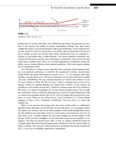
FIGURE 11.6
Reliability Index; B X Life (L BX ).

product that are weaker than other sites. Reliability specialists can presume the loca-
tion of the weakest site and/or its failure mechanisms, though they don’t know
whether the failure will actually happen in the targeted lifetime, or how high the fail-
ure rate would be. So if we extract one or two failure sites in the product, mostly in a
given module or unit, and classify their failure mechanisms into two categories—
lifetime L B and failure rate λ within lifetime—the factors related to reliability esti-
mation are decreased, and the cases pertaining to moderately large factors become
small-factor-number cases. Thus, we can make quantitative estimations about reli-
ability issues—mainly lifetime under normal conditions. This is the simple explana-
tion to understand CEOs.
Let’s describe in common sense terms the basic concepts of the required statis-
tics and methods pertaining to establish the quantitative lifetime specification,
which CEOs can easily understand as seen in Figure 11.6. For instance, take auto-
mobiles. Assume that we test 100 cars in Germany for 10 years and find no trouble
(10 years, 160,000 km). We can conclude that the car’s failure rate is below 1% per
10 years, which is called “B 1 life 10 years,” using a common sense level of con-
fidence. When we conclude that the car’s failure rate is below 1% per 10years, its
confidence level reaches around 60%, called the common sense level of confidence.
Of course, we cannot test products for 10 years before market release. So we make
the accelerated vehicle testing by imposing heavy loads and high temperature until
we reach an acceleration factor (AF) of 10. This will reduce the test period by one-
tenth, or 1 year. Thus, we test 100 items for 1 year (16,000 km), or 1 week without
stoppage (7 days 24 h 100 km/h¼16,800 km). The next step is to reduce the
sample size.
Then, if you increase the testing time, the items would achieve a sufficiently
degraded state and many would fail after the test; therefore, we can greatly reduce
the sample size, because one or two failed samples would yield enough data to iden-
tify the problem area and make corrective action plans. Increasing the test time by
four times, or to 1 month, reduces the necessary sample size by the square of the
inverse of the test-time multiplier, to one-sixteenth (square of one-quarter), or six
engines. The final test specification, then, is that six engines should be tested for
1 month under elevated load and temperature conditions with the criterion that no
failure is found. This concept, called parametric accelerated life testing (parametric
ALT), is the key to reliability quantitative estimations.