Page 176 - Hardware Implementation of Finite-Field Arithmetic

m
Operations over GF ( p ) 159

a := product_mod_f(e, a, f);
for j in 0 .. m-1 loop e(J) := (a(J)*Frobenius(j,2))
mod P; end loop;
a := product_mod_f(e, a, f);
for j in 0 .. m-1 loop e(J) := (a(J)*Frobenius(j,4))
mod P; end loop;
a := product_mod_f(e, a, f);
for j in 0 .. m-1 loop e(J) := (a(J)*Frobenius(j,8))
mod P; end loop;
a := product_mod_f(e, a, f);
for j in 0 .. m-1 loop e(J) := (a(J)*Frobenius(j,1))
mod P; end loop;
A := Product_Mod_F(E, H, F);
e := Product(E, invert(a(0)));
Z := Product_Mod_F(e, G, F);

An executable Ada file oef2.adb, including Algorithm 6.8, in the
17
particular case where p = 239 and f(x) = x − 2, is available at
www.arithmetic-circuits.org.
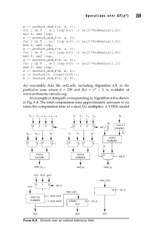
An example of datapath corresponding to Algorithm 6.8 is shown
in Fig. 6.4. The total computation time approximately amounts to six
times the computation time of a mod f(x) multiplier. A VHDL model

f m –1 1 f m –1 2 f m –1 4 f m –1 8 f 1 1 f 1 2 f 1 4 f 18 a 0

e 0
mod p
0 1 2 3 0 1 2 3 sel_f
........ inverter
–1
–1 –1 a 0
a m–1 e m–1 a 0 a 1 e 1 a 0
mod p
multiplier
0 1 0 1 0 1 0 1
a 0
mod p mod p 0 1
multiplier multiplier sel_e

next_e m–1
next_e 1 next_e 0
a(x) h(x) g(x)
next_e(x)
0 1 2
e(x) sel_a
ce ce_e
next_a(x)
start_mult
mod f(x)
multiplier
mult_done initially: ce ce_a
h(x)
z(x) a(x) e(x)

FIGURE 6.4 Division over an optimal extension fi eld.