Page 174 - Hardware Implementation of Finite-Field Arithmetic

m
Operations over GF ( p ) 157

Property 6.1 In an OEF
ax() p () i = a f x m–1 + a f x m–2 + ... + aaf
m–1 m–1 i m–2 m–2 i 00 i
jt
i
with f = c mod p and t = ⎣p /m⎦
ji
Proof Taking into account that a = a for any a in Z (Fermat’s little
p
p
p
p
p
theorem) and that (α + β) = α + β for any α and β belonging to a finite
field of characteristic p, one deduces that
+
i
p
p
p
m
a p () = a,∀a ∈ Z and (αβ ) () i = α () i + β () i , ∀α and β ∈ GF(p )
p
Thus
+
(a x m–1 + a x m–2 + ... + a x a ) p () i
m–1 m–2 1 0
= a x (m–1) p i + a x ( m–2) p i + ... + a x p ( ) + a
i
m
m–1 m–2 1 0
Then, according to Eq. (6.28), p ≡ 1 mod m, that is, p = tm + 1,
i
i
so that
j
jt
j
)
a x jp i = ax ( tm+1 ) j = ax ( m jt x = a c x = a f x j j
j j j j jji
The Frobenius constants f can be computed in advance so that, in
ji
Algorithm 6.6, the computation of h(x) r − 1 , that is,
p
hx () r–1 = hx hx () p ( 2 ) ... hx () p ( m–1 )
()
can be computed using Property 6.1. In the following algorithm the
function frobenius( j, i) returns f .
ji
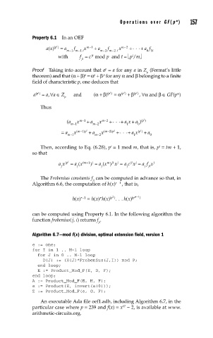
Algorithm 6.7—mod f(x) division, optimal extension field, version 1
e := one;
for I in 1 .. M-1 loop
for J in 0 .. M-1 loop
D(J) := (H(J)*Frobenius(J,I)) mod P;
end loop;
E := Product_Mod_F(E, D, F);
end loop;
A := Product_Mod_F(E, H, F);
e := Product(E, invert(a(0)));
Z := Product_Mod_F(e, G, F);

An executable Ada file oef1.adb, including Algorithm 6.7, in the
particular case where p = 239 and f(x) = x − 2, is available at www.
17
arithmetic-circuits.org.