Page 242 - Hardware Implementation of Finite-Field Arithmetic

222 Cha pte r Se v e n

It was proven in [RH04] that the following equalities hold:
−
e () 0 + e ( ) 1 = h ; m k ≤ ≤ m 2−
j
+
j j j k 2 − m 2 (7.68)
j
e () 2 + e ( ) 3 = e 0 () + e 1 ( ) ; k ≤ ≤ m − 1
−
−
j
3
j
j jk 2 jk 2
T
Let e (01 ) , 0 ≤ j ≤ m – 1, represent the elements of (P + P ) E, where P
j 0 1 0
and P are the submatrices shown in Fig. 7.10a and 7.10b, respectively.
1
Then, substituting t = 3 in Eq. (7.54) and using Eq. (7.68), the coordi-
T
nates of the product C = AB given in Eq. (7.29) as C = D + P E can be
found as follows [RH04]:
c = d + e (01 ) + e (01 ) ; 0 ≤ j ≤ m − 1
−
j j j j k 2 (7.69)
( )
01
where e = 0 for j < k and
−
jk 2
2
⎧ e ; 0 ≤≤ k − 1
() 0
j
⎪ j 1
e ⎪ () 0 + e ; k ≤ ≤ m − k − 1
( ) 1
j
1
e (01 ) = ⎨ j j 1 2 (7.70)
j m − k ≤ ≤ m −
⎪ h jk − m ; 2 j 2
+
2
⎪ e ; j = m − 1
1 ()
⎩ j
8
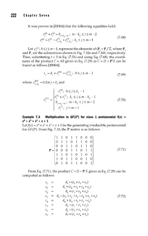
Example 7.3 Multiplication in GF(2 ) for class 1 pentanomial f(x) =
8
3
5
x + x + x + x + 1
Let f(x) = x + x + x + x + 1 be the generating irreducible pentanomial
3
8
5
8
for GF(2 ). From Fig. 7.10, the P matrix is as follows:
⎛ 11 0 11 000⎞
⎜ 0 11 0 11 00 ⎟
⎜ ⎟
⎜ 00 11 0 11 0 ⎟
⎜
P = 000 11 0 11 ⎟ (7.71)
⎜ 1 1 01 01 01 ⎟
⎜ ⎟
1001 1 0 01 0
⎜ ⎝ 01 01 1 0 01⎠ ⎟

T
From Eq. (7.71), the product C = D + P E given in Eq. (7.29) can be
computed as follows:
c = d + ( e + e + e )
0 0 0 4 5
c = d + ( e + e + e + )
e
1 1 0 1 4 6
c = d + ( + e + e )
e
2 2 1 1 2 5
c = d + e ( + e + e + e + e + e ) (7.72)
3 3 0 2 3 4 5 6
+
c = d + e ( + e + e + e )
4 4 0 1 3 6
c = d + e ( + e + e )
5 5 1 2 4
c = d + e ( + e + e )
6 6 2 3 5
c c = d + ( e + e + )
e
7 7 3 4 6