Page 110 - Industrial Ventilation Design Guidebook

4,2 STATE VALUES OF HUMID AIR; MOLLIER DIAGRAMS AND THEIR APPLICATIONS 75

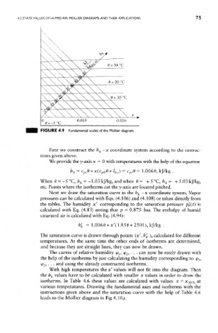
FIGURE 4.9 Fundamental scales of the Molfier diagram.

First we construct the h k-x coordinate system according to the instruc-
tions given above.
We provide the y-axis x = 0 with temperatures with the help of the equation
h = c e + x(c e+i ) = e = 1.0060, kj/kg .
pt
k
Cpi
ph
ho
When 0 = -5 °C, b k = -5.03 kj/kg, and when 0= + 5°C,h k = + 5,03 kj/kg,
etc. Points where the isotherms cut the y-axis are located pitched.
Next we draw the saturation curve in the h k - x coordinate system. Vapor
pressures can be calculated with Eqs. (4.106) and (4.108) or taken directly from
the tables. The humidity x' corresponding to the saturation pressure ph(t) is
calculated with Eq. (4.83) noting that p = 0.875 bar. The enthalpy of humid
saturated air is calculatted with Eq. (4.94):
h' k = 1.0060 + x'(1.850 + 2501),kJ/kg .

The saturation curve is drawn through points (x', b' k ), calculated for different
temperatures. At the same time the other ends of isotherms are determined,
and because they are straight lines, they can now be drawn.
The curves of relative humidity <p l5 <p 2, . . . can now be easily drawn with
the help of the isotherms by just calculating the humidity corresponding to 9 J5
<P2, • . . and using the already constructed isotherms.
With high temperatures the x' values will not fit into the diagram. Then
the h k values have to be calculated with smaller x values in order to draw the
isotherms. In Table 4.6 these values are calculated with values x = X$Q% at
various temperatures. Drawing the fundamental axes and isotherms with the
instructions given above and the saturation curve with the help of Table 4.6
leads to the Mollier diagram in Fig 4.100.