Page 101 - Integrated Wireless Propagation Models

M a c r o c e l l P r e d i c t i o n M o d e l s - P a r t 1 : A r e a - t o - A r e a M o d e l s 79

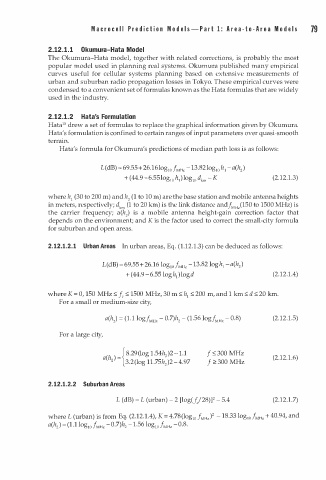
2 . 1 2 . 1 . 1 Okumura-Hata Model
The Okumura-Hata model, together with related corrections, is probably the most
popular model used in planning real systems. Okumura published many empirical
curves useful for cellular systems planning based on extensive measurements of
urban and suburban radio propagation losses in Tokyo. These empirical curves were
condensed to a convenient set of formulas known as the Hata formulas that are widely
used in the industry.

2.12.1.2 Hata's Formulation
1
5
Hata drew a set of formulas to replace the graphical information given by Okumura.
Hata's formulation is confined to certain ranges of input parameters over quasi-smooth
terrain.
Hata's formula for Okumura's predictions of median path loss is as follows:

L ( dB) = 69.55+ 26.1 6 l og10 fMHz -13.82 l og10 /; -a(h2)
+ ( 44.9-6.55log10/;) l og10 dkm -K (2.12.1.3)

where h1 (30 to 200 m) and h2 (1 to 10 m) are the base station and mobile antenna heights
in meters, respectively; dkm (1 to 20 km) is the link distance and fMHz(150 to 1500 MHz) is
the carrier frequency; a(h) is a mobile antenna height-gain correction factor that
depends on the environment; and K is the factor used to correct the small-city formula
for suburban and open areas.

2.12.1. . 1 Urban Areas In urban areas, Eq. (1.12.1.3) can be deduced as follows:
2
L ( dB) = 69.55+ 26.16 log10 fMHz -13.82 logh1 -a(h2)
+ (44.9 6 .55 logh1) l ogd (2.12.1.4)
-
d
where K = 0, 150 MHz ::; fc ::; 1500 MHz, 30 m ::; h1 ::; 200 m, and 1 km::; ::; 20 km.
For a small or medium-size city,
a(hz) = (l.l logf M Hz - 0.7)h2 - (1.56 logfMHz - 0.8) (2.12.1.5)

For a large city,

{ 8.29 ( log 1.54h2)2 - 1 .1 f ::; 3 00 MHz
1 1
a(h ) = 3.2(log .75h2)2-4.97 f � 3 00 MHz (2.12. . 6)
1
2
2.12.1.2.2 Suburban Areas
2
L (dB) = L (urban) - 2 [log(.f/ 2 8)] - 5.4 (2.12.1.7)
2
where L (urban) is from Eq. (2.12.1.4), K = 4.78(log10 f M HJ - 18.33 log10 f M Hz + 40.94, and
a(h2) = (l.l log10 f M Hz -0.7)h2 -1 . 56 log10 fMHz -0.8.