Page 157 - Integrated Wireless Propagation Models

M a c r o c e l l P r e d i c t i o n M o d e l s - P a r t 2 : P o i n t - t o - P o i n t M o d e l s 135

The brief notations shown in Fig. 3.1.6.3.1 stand for following:

=
TxHt b ase station antenna height + above mean sea level (AMSL) [ft]
MoHt = mobile antenna height
HtAGL b ase station antenna elevation above ground level [ft]. The antenna height
=
in the standard condition is 100 ft. If the actual height h1 is not 100 ft, a gain difference
20 log (h1 /100) should be added to the final prediction value.
OAL = open area loss. If the default
FSL = free space loss
T b ase station transmitter
=
L = land
W = water

If the standard condition (see Sec. . 1 . 2.1) is applied, the OAL includes a loss slope
3
of 43.5 dB I decade and 1-mile intercept of -49 dBm, and the FSL equation uses the total
ERP (antenna output power and gain) to be 46 dBm at the base station.
The shadow loss is obtained from Sec. 3.1.2.4.
Four situations of the mobile locations:
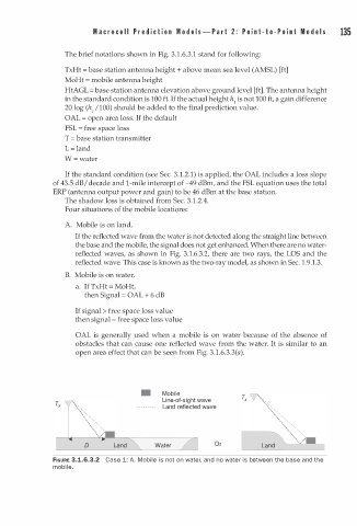
A Mobile is on land.
If the reflected wave from the water is not detected along the straight line between
the base and the mobile, the signal does not get enhanced. When there are no water­
reflected waves, as shown in Fig. 3.1.6.3.2, there are two rays, the LOS and the
reflected wave. This case is known as the two-ray model, as shown in Sec. 1.9.1.3.

B. Mobile is on water.
a. If TxHt = MoHt,
then Signal = OAL + 6 dB
If signal > free space loss value
then signal = free space loss value
OAL is generally used when a mobile is on water because of the absence of
obstacles that can cause one reflected wave from the water. It is similar to an
open area effect that can be seen from Fig. 3.1.6.3.3(a) .

• Mobile
Line-of-sight wave Tx Y'' ,
Land reflected wave , ,' ' , ,
,
'
.----- _[__ ________ ' , , ,' , , ,' , ,

0 Water Or Land , , ' , , , ,/"'
FIGURE 3.1.6.3.2 Case 1: A. Mobile is not on water, and no water is between the base and the
mobile.