Page 311 - Integrated Wireless Propagation Models

I n - B u i l d i n g ( P i c o c e l l ) P r e d i c t i o n M o d e l s 289

The received signal inside the room is

Wall (5.2.8.3.2)
og r +
LOS
LOS
_ " " loss, -�i=l m 1 [( d ) ! d )]
" "
- P LOS - �i=l mill wall ; room
where P, = received power in dBm in the room,
Pws = the power at the interception point of LOS and the first wall in dBm,
n = n umber of walls,
= the path-loss slope for each wall in dB I dec (obtained in Sec. 5.3.2.1 ),
m ill wa n
Wall = l oss due to the ith wall,
loss
;
r = the mobile radial distance from the base transmitter to the mobile receiver
in meters,
m room = the path-loss slope for inside the room in dB/ dec, and
dws = LOS distance from the transmitter to the first wall in meters.
= L o is
The general formula of the Lee model is shown in Sec. 5.3.5, where L ill wa n ( )
expressed in Eq. (5.2.8.3.2).
5.2.8.3.2 Measurement Integration The success of any prediction model relies on taking
advantage of field measurement data and fine-tuning the model formula for different
environments. Due to the enhancement on the Lee model, the four curves shown in
Fig. 5.2.8.3.3 can be adjusted through measurement integration.
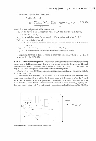
As shown in Fig. 5.2.8.3.7, different setups are used in collecting measured data to
tune the Lee model.
The first one will be in the LOS situation. In the LOS situation, two different cases
need to be specified. One is within the Fresnel zone, and the other is after the Fresnel
zone area. This needs to be distinguished so that behavior after the close-in distance can
be further fine-tuned. Based on the measured data for handling this category, the path­
loss curve can be derived. The various path-loss setups are highlighted in Fig. 5.2.8.3.8.

e LOS
0
o Non-LOS aggregate

FIGURE 5.2.8.3.7 Measurement data collection.