Page 314 - Integrated Wireless Propagation Models

292 C h a p t e r F i v e

Between these two wings, there is a corridor junction, which is 8 x 10 m in length
and width, as shown in Fig. 5.3.2.0.2. On each floor, the brick walls were used to divide
several classrooms (three classrooms in the north wing and three classrooms in the
south wing) and an aisle. The furniture in the classroom includes school desks and
chairs, which were made of plastic and reinforced metal brackets. Both the north and
the south sidewalls were full of windows. There were three access points (AP) in the
north and south wings on each floor. The three APs were operational on three signal
channels: channels 1, 6, and 11. The APs were mounted fixed at a height of . 5 m.
1
5.3.2. 1 A Same-Floor Case
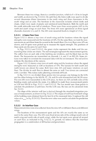
Figure 5.3.2.1.1 shows a top view of south wing and the locations where the signal
strengths were measured and the locations of APs. On the same floor, we took the mea­
surements on each floor from the second to the fourth floor. On every floor, nine APs are
shown, and 18 spots were picked up to measure the signal strength. The positions of
these spots are the same for each floor.
In Figs. 5.3.2.1.1 and 5.3.2.1.2, the green circles represent the desks and the sur­
rounding blue circles are chairs. The red rectangles represent the measurement points.
The yellow bars on each side of the building are windows, and the black bars are the
doors. The frequencies are transmitted on channels 1, 6, and 11 on 802.11b. Some pic­
tures were taken to correlate the measured data with the environment. The red arrows
indicate the directions of the camera.
Figure 5.3.2.1.2 shows a top view of north wing and the locations where the signal
strengths were measured as well as locations of APs. The layouts for both south and
north towers are almost the same. Both have nine APs and many windows on each
floor. The divider in each floor is almost the same as well. Two towers are connected
with a corridor. This makes radio planning extremely difficult.
In Fig. 5.3.2.1.2, we divided these points into two groups: one belongs to the LOS,
and the other belongs to the NLOS. P2 , P4, and P6 were transmitted into NLOS areas.
The rest APs were transmitted in the LOS areas. As there are APs on both sides of the
building inside and outside the room, it is difficult to mark these measurement points
as LOS and NLOS in Figs. 5.3.2.1.1 and 5.3.2.1.2. The Lee model uses these points to
calculate the prediction of path loss. For the LOS case, the loss can be calculated from
Sec. 5.2.2.1 .
o
The slope f the interior wall loss s derived through the standard integration pro­
i
cess of measurement, as shown in Fig. 5.3.2. . 3. The slopes of wall loss from both wings
1
of the building were obtained from the best fit of the measured data. It replaced the old
value of min wall in Eq. (5.2.8.3.2). Then the new value was used to calculate the prediction
values.
5.3.2.2 An lnterfloor Case
Measurement data were also collected from the nine APs at different floors and different
wings.
The locations of the measurement spots and the APs are exactly the same as we
used in the same-floor case. The APs were fixed at one side of the ceilings (south side of
north wing and north side of south wing), while the test spots were spread all around
on each floor, as indicated in Fig. 5.3.2.1.2. In general, we believe that the interfloor
propagation is a combination of diffraction and penetration.