Page 75 - Integrated Wireless Propagation Models

M a c r o c e l l P r e d i c t i o n M o d e l s - P a r t 1 : A r e a - t o - A r e a M o d e l s 53

O r-----------------------�-------,

m
:s.
gJ
.2 ••• .••
..c Plane : ... · .... ···· :,
h
� eart loss �
______ --��
_100 � -+ -� r__ , � ,·� · -�---�
�
· ·
·
·. :::·· . L_ Free space
..
···· ····· ···· i..
· . · . L ·
: .. .. . ...
: � .. ..
.
..
-150 �-- -- -- ---- -- -a -- -- -- -- -- --------�
.. . .
1 0 1 1 0 2 1 0 3 1 0 4
Distance (m)
M
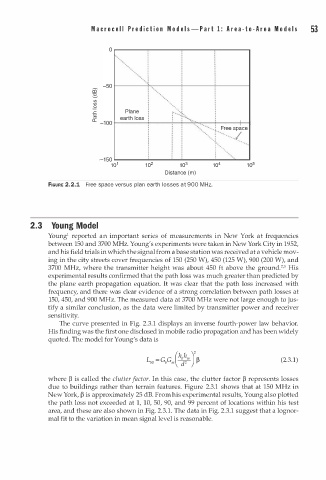
FIGURE 2.2.1 Free space versus plan earth losses at 900 H z.
2.3 Y o u n g Model
1
Young reported an important series of measurements in New York at frequencies
between 150 and 3700 MHz. Young's experiments were taken in New York City in 1952,
and his field trials in which the signal from a base station was received at a vehicle mov­
ing in the city streets cover frequencies of 150 (250 W), 450 (125 W), 900 (200 W), and
2
3700 MHz, where the transmitter height was about 450 ft above the ground. •3 His
experimental results confirmed that the path loss was much greater than predicted by
the plane earth propagation equation. It was clear that the path loss increased with
frequency, and there was clear evidence of a strong correlation between path losses at
150, 450, and 900 MHz. The measured data at 3700 MHz were not large enough to jus­
tify a similar conclusion, as the data were limited by transmitter power and receiver
sensitivity.
The curve presented in Fig. 2.3.1 displays an inverse fourth-power law behavior.
His finding was the first one disclosed in mobile radio propagation and has been widely
quoted. The model for Young's data is

(2.3.1)

where � is called the clutter a ctor. In this case, the clutter factor � represents losses
f
due to buildings rather than terrain features. Figure 2.3.1 shows that at 150 MHz in
New York, � is approximately 25 dB. From his experimental results, Young also plotted
the path loss not exceeded at 1, 10, 50, 90, and 99 percent of locations within his test
1
area, and these are also shown in Fig. 2.3. . The data in Fig. 2.3.1 suggest that a lognor­
mal fit to the variation in mean signal level is reasonable.