Page 203 - Introduction to Autonomous Mobile Robots

188

∆s + ∆s l  ∆s ∆– s l  Chapter 5
r
r
----------------------cos  θ + ------------------- 
2 2b
x ∆s ∆– s
,,
(
,
r
,
r
p' = fxy θ∆s ∆s ) = y + ∆s + ∆s l   θ + ------------------- l   (5.7)
----------------------sin
l
r
2b
θ 2
∆s ∆– s l
r
-------------------
b
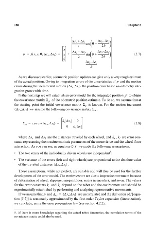
As we discussed earlier, odometric position updates can give only a very rough estimate
of the actual position. Owing to integration errors of the uncertainties of and the motion
p
errors during the incremental motion ∆s ∆s;( r l ) the position error based on odometry inte-
gration grows with time.
p'
In the next step we will establish an error model for the integrated position to obtain
the covariance matrix Σ p' of the odometric position estimate. To do so, we assume that at
the starting point the initial covariance matrix Σ p is known. For the motion increment
( ∆s ∆s ) we assume the following covariance matrix Σ :
;
r l ∆
k ∆s r 0
,
(
r
Σ = covar ∆s ∆s ) = (5.8)
∆
r
l
0 k ∆s
l l
where ∆s r and ∆s l are the distances traveled by each wheel, and k r , k l are error con-
stants representing the nondeterministic parameters of the motor drive and the wheel-floor
interaction. As you can see, in equation (5.8) we made the following assumptions:
5
• The two errors of the individually driven wheels are independent ;
• The variance of the errors (left and right wheels) are proportional to the absolute value
of the traveled distances ∆s ∆s;( . )
r l
These assumptions, while not perfect, are suitable and will thus be used for the further
development of the error model. The motion errors are due to imprecise movement because
of deformation of wheel, slippage, unequal floor, errors in encoders, and so on. The values
for the error constants k and k depend on the robot and the environment and should be
r l
experimentally established by performing and analyzing representative movements.
If we assume that and ∆ rl = ( ∆s ∆s ) are uncorrelated and the derivation of f [equa-
;
p
l
r
tion (5.7)] is reasonably approximated by the first-order Taylor expansion (linearization),
we conclude, using the error propagation law (see section 4.2.2),
5. If there is more knowledge regarding the actual robot kinematics, the correlation terms of the
covariance matrix could also be used.