Page 204 - Introduction to Autonomous Mobile Robots

189
Mobile Robot Localization
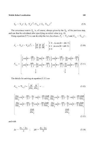
Σ p' = ∇ f Σ ⋅ ∇ f + ∇ ∆ rl f Σ ⋅ ∇ ∆ rl f T (5.9)
⋅
T
⋅
∆
p
p
p
The covariance matrix Σ p is, of course, always given by the Σ p' of the previous step,
and can thus be calculated after specifying an initial value (e.g., 0).
Using equation (5.7) we can develop the two Jacobians, F = ∇ f and F = ∇ : f
p p ∆ ∆
rl rl
⁄
10 ∆ssin ( θ + ∆θ 2)
–
T f ∂ ∂ ∂ f
f
F = ∇ f = ∇ f() = ----- ----- ------ = ( ∆θ 2) (5.10)
⁄
p p p 01 ∆scos θ +
x ∂ ∂ y θ∂
00 1

1  ∆θ  ∆s  ∆θ 1  ∆θ  ∆s  ∆θ 
---cos  θ + ------- – ------sin  θ + ------- ---cos  θ + ------- + ------sin  θ + -------
2 
2 
2 
2 
2 2b 2 2b
F ∆ = 1  ∆θ  ∆s  ∆θ  1  ∆θ  ∆s  ∆θ  (5.11)
-------
-------
-
------- –
------- +
------ cos
rl ---sin  θ + 2  ------cos  θ + 2  --sin  θ +  θ + 2 
2 2b 2 2  2b
1 1
--- – ---
b b
The details for arriving at equation (5.11) are
f ∂
f ∂
F ∆ = ∇ ∆ f = ----------- ---------- = … (5.12)
rl rl ∂ ∆s ∂ ∆s
r l
∂ ∆s  ∆θ  ∆s  ∆θ  ∆θ∂ ∂ ∆s  ∆θ  ∆s  ∆θ  ∆θ∂
–
–
+
+
-------------cos θ ------ + ------ sin θ ------ ------------- ------------cos θ ------ + ------ sin θ ------ ------------
+
+
∂ ∆s  2  2  2  ∂ ∆s ∂ ∆s  2  2  2  ∂ ∆s
r r l l
∂ ∆s  ∆θ  ∆s  ∆θ  ∆θ∂ ∂ ∆s  ∆θ  ∆s  ∆θ  ∆θ∂
+
+
+
+
-------------sin  θ ------ + ------cos  θ ------ ------------- ------------sin  θ ------ + ------cos  θ ------ ------------
∂ ∆s 2  2 2  ∂ ∆s ∂ ∆s 2  2 2  ∂ ∆s
r r l l
∂ ∆θ ∂ ∆θ
------------- ------------
∂ ∆s ∂ ∆s
r l
(5.13)
and with
∆s + ∆s l ∆s ∆– s l
r
r
∆s = ---------------------- ; ∆θ = ------------------- (5.14)
2 b