Page 99 - Introduction to Autonomous Mobile Robots

84

3.6.2.2 Kinematic model Chapter 3
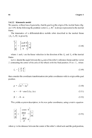
We assume, without loss of generality, that the goal is at the origin of the inertial frame (fig-
ure 3.19). In the following the position vector xy θ,,[ ] T is always represented in the inertial
frame.
The kinematics of a differential-drive mobile robot described in the inertial frame
{ X Y θ} is given by
,
,
I
I
I
x · cos θ 0
· v
y = sin θ 0 ω (3.48)
θ · 0 1
·
·
x
where and are the linear velocities in the direction of the X I and Y I of the inertial
y
frame.
Let denote the angle between the x axis of the robot’s reference frame and the vectorα R
ˆ x connecting the center of the axle of the wheels with the final position. If α ∈ I , where
1
 π π
--- ---
I = – , (3.49)
1  2 2
then consider the coordinate transformation into polar coordinates with its origin at the goal
position.

2 2
ρ = ∆x + ∆y (3.50)

(
,
α = – θ + atan 2 ∆y ∆x) (3.51)
–
β = – θ α (3.52)
This yields a system description, in the new polar coordinates, using a matrix equation

ρ · – cos α 0
α
v
sin
·
α = ----------- – 1 ω (3.53)
ρ
β · sin α
– ----------- 0
ρ
ρ
where is the distance between the center of the robot’s wheel axle and the goal position,