Page 101 - Introduction to Autonomous Mobile Robots

86

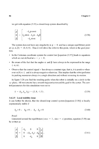
we get with equation (3.53) a closed-loop system described by Chapter 3

ρ · k – ρcos α
ρ
·
α
α = k sin – k α – k β (3.58)
α
β
ρ
β · k – ρ sin α
The system does not have any singularity at ρ = 0 and has a unique equilibrium point
,,
at ρ α β,,( ) = ( 00 0) . Thus it will drive the robot to this point, which is the goal posi-
tion.
• In the Cartesian coordinate system the control law [equation (3.57)] leads to equations
which are not defined at x = y = . 0
α
β
• Be aware of the fact that the angles and have always to be expressed in the range
,
– ( π π) .
• Observe that the control signal has always a constant sign, that is, it is positive when-
v
ever α 0() ∈ I and it is always negative otherwise. This implies that the robot performs
1
its parking maneuver always in a single direction and without reversing its motion.
In figure 3.20 you find the resulting paths when the robot is initially on a circle in the
xy plane. All movements have smooth trajectories toward the goal in the center. The con-
trol parameters for this simulation were set to

,
,
,,
k = ( k k k ) = ( 38 – 1.5) . (3.59)
β
ρ
α
3.6.2.5 Local stability issue
It can further be shown, that the closed-loop control system [equation (3.58)] is locally
exponentially stable if
k > 0 ; k < 0 ; k – k > 0 (3.60)
α
ρ
β
ρ
Proof:
Linearized around the equilibrium ( cos x = 1 , sin x = x ) position, equation (3.58) can
be written as

ρ · k – ρ 0 0 ρ
·
k
α = 0 – ( k – ) k– β α , (3.61)
ρ
α
β · 0 k – ρ 0 β