Page 406 - Introduction to Information Optics

7.5. Pattern Recognition Using Composite Filtering 39 1.

2. Noneffective pixels are randomly assigned with equal probability within
the interval [-N, N], where n - 0, ± 1, ±2, . . . , ± N, and 2N + 1 is the
number of quantized gray levels.
3. Assign the desired correlation profiles for the target and the antitarget
l
a
sets (i.e., W and W ).
4. Set a desired allowable error value (e.g., a 1 % error rate is used).
5. Assume the initial QCF has 2N + 1 randomly distributed gray levels,
and the initial system temperature is T. For example, the initial kT for
the desired correlation energy is given in step 3.
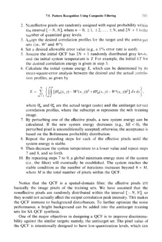
6. Calculate the initial system energy E, which can be determined by its
mean-square-error analysis between the desired and the actual correla-
tion profiles, as given by

2
a
2
E - M"(JC, >')) + (0" m(*, y) - W (x, .y)) ] dx dy
= Z j (T
w= l UJ
where 0^ and 0£, are the actual target (auto) and the antitarget (cross)
correlation profiles, where the subscript m represents the mth training
image.
7. By perturbing one of the effective pixels, a new system energy can be
calculated. If the new system energy decreases (e.g., A£ < 0), the
perturbed pixel is unconditionally accepted; otherwise, the acceptance is
based on the Boltzmann probability distribution.
8. Repeat the preceding steps for each of the effective pixels until the
system energy is stable.
9. Then decrease the system temperature to a lower value and repeat steps
7 and 8, and so forth.
1 0. By repeating steps 7 to 9, a global minimum energy state of the system
(i.e., the filter) will eventually be established. The system reaches the
stable condition as the number of iterations increases beyond 4 x M,
where M is the total number of pixels within the QCF.

Notice that the QCF is a spatial-domain filter; the effective pixels are
basically the image pixels of the training sets. We have assumed that the
noneffective pixels are randomly distributed within the interval [ — JV, ATJ, so
they would not actually affect the output correlation peak intensity. This makes
the QCF immune to background disturbances. To further optimize the noise
performance, a bright background can be added into the antitarget training
sets for SA QCF synthesis.
One of the major objectives in designing a QCF is to improve discrimina-
bility against the similar targets; namely, the antitarget set. The pixel value of
the QCF is intentionally designed to have low-quantization levels, which can