Page 180 - Introduction to Mineral Exploration

8: EXPLORATION GEOCHEMISTRY 163

association reflecting hydrothermal alteration
or even element depletion. Anomalies are l
defined by statistically grouping data and 2.72 l A:12.6%
comparing these with geology and sampling l l
l
information. Normally this grouping will be l l
undertaken by computer and a wide variety of 2.24 l l
statistical packages are available; for micro- Log (ppm) l l
computers, one of MINITAB, SYSTAT, and 1.76 l l
STATISTICA is recommended at a cost of l l l
$US200–500 each. B:87.4% l l
The best means of statistically grouping data 1.28 l l
is graphical examination using histograms and Cu l l
box plots (Howarth 1984, Garrett 1989). This
is coupled with description using measures of 0.80 99 95 85 70 50 30 15 5 1
central tendency (mean or median) and of stat- Cumulative (%)
istical dispersion (usually standard deviation).
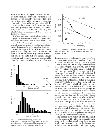
It would be expected that if data are homo- FIG. 8.5 Probability plot of the Daisy Creek copper
genous then they will form a continuous data. The data have been subdivided into two log
normal or, more likely, log-normal distribu- normal groups.
tion but if the data fall into several groups
then they will be multi-modal as shown in the determinations of soil samples from the Daisy
example in Fig. 8.4. These are a set of copper Creek area of Montana and have been described
in detail by Sinclair (1991). The histogram
shows a break (dip) in the highly skewed data
100
(a)
at 90 and 210 ppm. This grouping can be well
seen by plotting the data with a probability
80
Frequency 60 scale on the x axis (Fig. 8.5); log-normal dis-
tributions form straight lines and multi-modal
groups form straight lines separated by curves
40
500 -980 (for full details see Sinclair 1976). The Daisy
20 Creek data show thresholds (taken at the upper
limit, 99%, of the lower subgroups) which can
0 be set at 100 ppm to divide the data into two
10 110 210 310 410 510 groups and at 71 and 128 ppm if three groups
Copper (ppm) are used. The relationship of the groups to
other elemental data should then be examined
(b) by plotting and calculating the correlation
40
matrix for the data set. In the Daisy Creek
example there is a strong correlation (0.765)
Frequency 30 between copper and silver (Fig. 8.6) which re-
flects the close primary association between
20
the two elements, whereas the correlation
between copper and lead is low (0.12) reflect-
10 ing the spatial displacement of galena veins
from chalcopyrite. If geological or sampling
0 data are coded it will be possible to compare
10 100 1000 these groups with that information.
Log (10) copper (ppm)
The spatial distribution of the data must
FIG. 8.4 Arithmetic and log 10 transformed then be examined by plotting elemental data
histograms of Daisy Creek copper data. Note the using the intervals that delineate the groups or
positive skew of the arithmetic histogram. For by plotting the data by percentiles (percentage
further discussion see text and Sinclair 1991. of data sorted into ascending order); 50, 75, 90,