Page 181 - Introduction to Mineral Exploration

164 C.J. MOON

(a) 1400
+ + + + + + + + +
+ + + + + + + + +
1200
+ + + + + + + + +
+ + + + + + + + + + + + + + + + + + + N
Lead (ppm) 1000 + + + + + + + + + + + + + + + + + + + + + + + + + + + + + + + + + + + + + + + + + + + + + + + + + + +
+
+
800
+
+
+
+
600
+
+
400 + + + + + + + + + + + + + + + + + + + + + + + + + + + + + +
+ + + + + + + + + + + + + + + + + + +
200 + + + + + + + + + + + +
Cu
+ + + + + + + + + + + + + +
0
+ + + + + + + + + + + Pb
(b) 2 + + + + + + + + + + + Ag
+ + + + + + + + +
+ + + + + + + + +
0 50 m
1.5 + + + + + + + + +
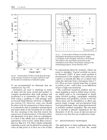
Silver (ppm) 1 FIG. 8.7 Contour plot of Daisy Creek data showing
the highest anomalous populations for copper
(>128 ppm), lead (>69 ppm), and silver (>0.55 ppm).
The relative size and relative positions of the
0.5
anomalous areas reflect the primary zoning in the
underlying prospect. (From Sinclair 1991.)
0
0 200 400 600 800 1000 by representing them by symbols, which are
Copper (ppm) easier to interpret. Typical symbols are given
by Howarth (1982). A more usual method of
FIG. 8.6 Scatter plots of Daisy Creek data showing presentation if the samples were collected on
(a) the strong correlation of copper and silver and a grid is to present the data as a contour plot
(b) the lack of correlation of lead and copper.
using the intervals from a histogram (Figs 8.7,
8.4). Plots are best colored from blue to green
95 are recommended for elements that are to yellow to red – cold to hot, as an indication
enriched (see Fig. 9.8). of low to high concentrations.
Geologists are used to thinking in terms The combined statistical analysis and ele-
of maps and the most useful end product to ment mapping is used to define areas of inter-
compare geochemical data with geology and est which need to be investigated in detail,
geophysics is to summarize the data in map using detailed geology, topography sampling
form using a gridding or GIS package such information, and, probably, a return to the site.
as Geosoft Oasis Montaj, ArcView, or MapInfo These areas can be classified as to their sug-
(see section 9.2). However, some care should gested origin, seepage, and precipitation from
be taken with the preparation of these maps as local groundwaters, from transported material,
it is extremely easy to prejudice interpretation or probable residual anomalies. The aim must
and many maps in the literature do not reflect be to provide a rational explanation for the
the true meaning of the data but merely the chemistry of all the areas of interest and not
easiest way of representing it. If the data reflect merely to say that they are of unknown origin.
the chemistry of an area, such as a catchment,
it is best if the whole area is shaded with an
appropriate color or tone, rather than contour- 8.4 RECONNAISSANCE TECHNIQUES
ing (e.g. Figs 8.8, 9.8). Data which essentially
represent a point can be plotted by posting the The application of these techniques has been
value at that point or if there are a lot of data discussed in section 4.2.2 but the actual