Page 250 - Introduction to Mineral Exploration

10: EVALUATION TECHNIQUES 233

(a)
160
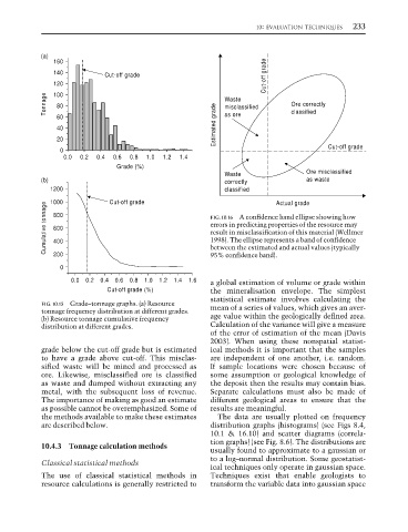
140 Cut-off grade Cut-off grade
120
Tonnage 100 Waste Ore correctly
80
misclassified
60 as ore classified
40 Estimated grade
20
0 Cut-off grade
0.0 0.2 0.4 0.6 0.8 1.0 1.2 1.4
Grade (%)
Waste Ore misclassified
(b) correctly as waste
1200 Cut-off grade classified Actual grade
1000
Cumulative tonnage 800 FIG. 10.16 A confidence band ellipse showing how

errors in predicting properties of the resource may
600
result in misclassification of this material (Wellmer
1998). The ellipse represents a band of confidence
400
200
95% confidence band).
0 between the estimated and actual values (typically
0.0 0.2 0.4 0.6 0.8 1.0 1.2 1.4 1.6 a global estimation of volume or grade within
Cut-off grade (%) the mineralisation envelope. The simplest
statistical estimate involves calculating the
FIG. 10.15 Grade–tonnage graphs. (a) Resource mean of a series of values, which gives an aver-
tonnage frequency distribution at different grades.
(b) Resource tonnage cumulative frequency age value within the geologically defined area.
distribution at different grades. Calculation of the variance will give a measure
of the error of estimation of the mean (Davis
2003). When using these nonspatial statist-
grade below the cut-off grade but is estimated ical methods it is important that the samples
to have a grade above cut-off. This misclas- are independent of one another, i.e. random.
sified waste will be mined and processed as If sample locations were chosen because of
ore. Likewise, misclassified ore is classified some assumption or geological knowledge of
as waste and dumped without extracting any the deposit then the results may contain bias.
metal, with the subsequent loss of revenue. Separate calculations must also be made of
The importance of making as good an estimate different geological areas to ensure that the
as possible cannot be overemphasized. Some of results are meaningful.
the methods available to make these estimates The data are usually plotted on frequency
are described below. distribution graphs (histograms) (see Figs 8.4,
10.1 & 16.10) and scatter diagrams (correla-
tion graphs) (see Fig. 8.6). The distributions are
10.4.3 Tonnage calculation methods
usually found to approximate to a gaussian or
to a log–normal distribution. Some geostatist-
Classical statistical methods
ical techniques only operate in gaussian space.
The use of classical statistical methods in Techniques exist that enable geologists to
resource calculations is generally restricted to transform the variable data into gaussian space