Page 253 - Introduction to Mineral Exploration

236 M.K.G. WHATELEY & B. SCOTT

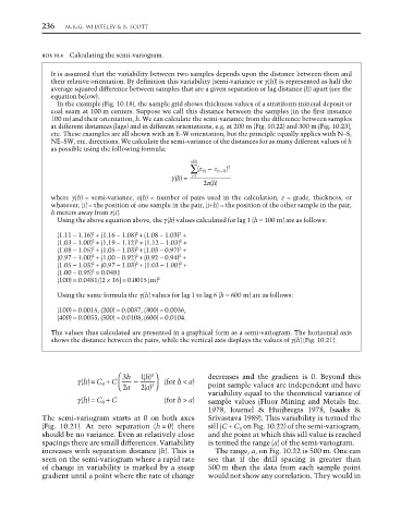
BOX 10.4 Calculating the semi-variogram.

It is assumed that the variability between two samples depends upon the distance between them and
their relative orientation. By definition this variability (semi-variance or γ (h)) is represented as half the
average squared difference between samples that are a given separation or lag distance (h) apart (see the
equation below).
In the example (Fig. 10.18), the sample grid shows thickness values of a stratiform mineral deposit or
coal seam at 100 m centers. Suppose we call this distance between the samples (in the first instance
100 m) and their orientation, h. We can calculate the semi-variance from the difference between samples
at different distances (lags) and in different orientations, e.g. at 200 m (Fig. 10.22) and 300 m (Fig. 10.23),
etc. These examples are all shown with an E–W orientation, but the principle equally applies with N–S,
NE–SW, etc. directions. We calculate the semi-variance of the distances for as many different values of h
as possible using the following formula:
nh
()
∑ (z − z (z h ) ) 2
−
()
i
=
γ () i=1
h
()
2 nh
where γ (h) = semi-variance, n(h) = number of pairs used in the calculation, z = grade, thickness, or
whatever, (i) = the position of one sample in the pair, (i+h) = the position of the other sample in the pair,
h meters away from z(i).
Using the above equation above, the γ (h) values calculated for lag 1 (h = 100 m) are as follows:
(1.11 − 1.16) + (1.16 − 1.08) + (1.08 − 1.03) +
2
2
2
(1.03 − 1.00) + (1.19 − 1.12) + (1.12 − 1.03) +
2
2
2
(1.08 − 1.05) + (1.05 − 1.03) + (1.03 − 0.97) +
2
2
2
(0.97 − 1.00) + (1.00 − 0.92) + (0.92 − 0.94) +
2
2
2
(1.05 − 1.03) + (0.97 − 1.03) + (1.03 − 1.00) +
2
2
2
2
(1.00 − 0.95) = 0.0481
(100) = 0.0481/[2 × 16] = 0.0015 (m) 2
Using the same formula the γ (h) values for lag 1 to lag 6 (h = 600 m) are as follows:
(100) = 0.0015, (200) = 0.0037, (300) = 0.0036,
(400) = 0.0055, (500) = 0.0108, (600) = 0.0104.
The values thus calculated are presented in a graphical form as a semi-variogram. The horizontal axis
shows the distance between the pairs, while the vertical axis displays the values of γ (h) (Fig. 10.21).
⎛ 3h 1h () ⎞ decreases and the gradient is 0. Beyond this
3
3 ⎟
γ (h) = C 0 + C ⎜ ⎝ − 2a () ⎠ (for h < a) point sample values are independent and have
2a variability equal to the theoretical variance of
γ (h) = C 0 + C (for h > a) sample values (Fluor Mining and Metals Inc.
1978, Journel & Huijbregts 1978, Isaaks &
The semi-variogram starts at 0 on both axes Srivastava 1989). This variability is termed the
(Fig. 10.21). At zero separation (h = 0) there sill (C + C 0 on Fig. 10.22) of the semi-variogram,
should be no variance. Even at relatively close and the point at which this sill value is reached
spacings there are small differences. Variability is termed the range (a) of the semi-variogram.
increases with separation distance (h). This is The range, a, on Fig. 10.22 is 500 m. One can
seen on the semi-variogram where a rapid rate see that if the drill spacing is greater than
of change in variability is marked by a steep 500 m then the data from each sample point
gradient until a point where the rate of change would not show any correlation. They would in