Page 108 - Introduction to Petroleum Engineering

ONE‐DIMENSIONAL WATER-OIL DISPLACEMENT 93
The water saturation at the intersection is the average water saturation
behind the front. The pore volume of oil produced at breakthrough equals the
average water saturation minus the initial water saturation. The volume of
water injected equals the volume of oil recovered at breakthrough; it also
equals the inverse of the slope of the tangent.
4. Postbreakthrough production behavior. Construct a tangent to the water
fractional flow curve for water saturation greater than S . The inverse of the
wf
slope of this tangent is the pore volume of water injected Q when the satura-
wi
tion at the tangent point reaches the producing well. Extrapolate the tangent to
intersect with the line f = 1. The water saturation at the intersection is the
w
average water saturation after injecting Q pore volume of water. The pore
wi
volume of oil produced Q equals the average water saturation minus the
op
initial water saturation S . Repeat step 4 as desired to produce additional oil
wi
recovery results.
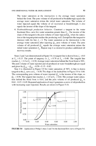
Steps 2 and 3 are demonstrated in Figure 5.8. A tangent line is drawn from f =00
.
w
.
.
.
at S = 015. The point of tangency is f wf = 078 at S wf = 048. The tangent line
wi
.
.
reaches f = 10 at S = 058. Average water saturation behind the flood front is 58%.
w
w
The pore volume of water injected and oil produced at water breakthrough are equal
−
.
.
and given by Q wibt = Q opbt =0580 15 = 043.
.
Step 4 is illustrated in Figure 5.9 for water saturation of 58%. A line is drawn
.
tangent to the f curve at S = 058. The slope of the dashed line in Figure 5.9 is 1.04.
w
w
The corresponding pore volume of water injected Q is the inverse of the slope, so
wi
.
Q = 096. The tangent line reaches f = 10 at S = 064. The average water satura-
.
.
w
w
wi
tion behind the flood front is 0.64, and the pore volume of oil produced Q is
op
0 64 015 = 0 49. Repeated application of step 4 generates a curve of oil production
−
.
.
.
with increasing water injection. Results are shown in Figure 5.10.
1.00
0.80 f wf = 0.78 S w,ave = 0.58
Water fraction flow 0.60 S wf = 0.48
0.40
0.20
0.00
0.00 0.20 0.40 0.60 0.80 1.00
Water saturation
FIgURE 5.8 Application of Welge’s steps 2 and 3 to the fractional flow curve of Figure 5.6.