Page 116 - Materials Chemistry, Second Edition

Will the well run dry? Developments in water resource planning and impact assessment

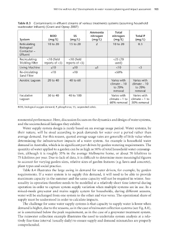
Table 8.3 Contaminants in effluent streams of various treatments systems (assuming household 103
wastewater influent) (Grant and Opray 2007)
Ammonia Total
BOD SS nitrogen nitrogen Total P
System (mg/L) (mg/L) (mg/L) (mg/L) (mg/L)
Reticulating 10 to 20 15 to 20 2 10 to 20 0.3
Biological
Contactor –
Effluent
Recirculating <10 (field <10 (field <25 (20
Trickling Filter reports of <5) reports of <5) used)
Living Machine ≤10 ≤10 ≤1 <10 <5
Re-circulating ≤10 ≤10 ≤50%
Sand Filter
Aerobic Lagoon 20 to 40 40 to 60 Varies with Varies with
climate – 10 climate – 10
to 20% to 20%
removal removal
Faculative 30 to 40 40 to 100 Varies with Varies with
Lagoon climate – 1 to climate – 1 to
60% removal 50% removal
BOD, biological oxygen demand; P, phosphorus; SS, suspended solids.

ronmental performance. Here, discussion focuses on the dynamics and design of water systems,
and the sociotechnical linkages they exhibit.
Water supply system design is rarely based on an average usage period. Water systems, by
their nature, will be sized according to peak demands for water over a period rather than
average demand. For this reason, quoted average usage rates are generally of little value when
determining the infrastructure impacts of a water system. An example is household water
demand in Australia, which is in significant part driven by garden watering requirements. The
quantity of water applied to a garden can be as high as 50% of total household water consump-
tion, although it is roughly 35% in the average Melbourne home, or about 70 kilolitres to
75 kilolitres per year. Due to lack of data, it is difficult to determine more meaningful figures
to account for varying garden sizes, relative sizes of garden features (e.g. lawn and concrete),
plant types and social practice.
Table 8.4 illustrates the large swing in demand for water driven, for example, by garden
requirements. If a water system is to supply this demand, it will need to be able to provide
maximum capacity in the summer and the same capacity will not be required in winter. Sea-
sonality in operation therefore needs to be modelled at a relatively short time interval during
operation in order to capture system supply variation when multiple systems are in use. In a
mixed-mode greywater and mains supply system for households, during different seasons,
water will be exchanged from one system to the other and vice versa. The operational share of
supply must be understood in order to calculate impacts.
The challenge for some water supply systems is that capacity to supply water is lower when
demand is higher, due to the seasons, as in the case of rainwater collection systems (see Fig. 8.8),
or is constrained below the peak requirement, as in the case of a greywater treatment system.
The rainwater collection example illustrates the need to undertake system analysis at a rela-
tively fine time interval (usually daily) to ensure supply and demand mismatches are properly
comprehended.

100804•Life Cycle Assessment 5pp.indd 103 17/02/09 12:46:21 PM