Page 176 - MATLAB an introduction with applications

Control Systems ——— 161

–3 Nyquist Diagram
×10
5
4
3
2
Imaginary Axis 1 0

–1
–2
–3
–4
–5
–3 –2 –1 0 1 2 3 4
Real Axis ×10 –3

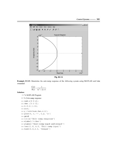
Fig. E3.14
Example E3.15: Determine the unit-ramp response of the following system using MATLAB and lsim
command.
()
Cs = 1
2
Rs 3s + 2s + 1
()
Solution:
>> % MATLAB Program
>> % Unit-ramp response
>> num =[0 0 1];
>> den =[3 2 1];
>> t=0:0.1:10;
>> r=t;
>> y =lsim(num,den,r,t);
>> plot(t, r,‘–’, t,y, ‘o’)
>> grid
>> title(‘Unit-ramp response’)
>> xlabel(‘t Sec’)
>> ylabel(‘Unit-ramp input and output’)
>> text(1.0, 4.0, ‘Unit-ramp input’)
>> text(5.0,2.0, ‘Output’)

F:\Final Book\Sanjay\IIIrd Printout\Dt. 10-03-09