Page 171 - MATLAB an introduction with applications

156 ——— MATLAB: An Introduction with Applications

>> fprintf(‘, Damping ratio=%g’, z)
>> fprintf(‘, Percent overshoot=%g’, Po*100)
>> fprintf(‘, Settling time=%g’, Ts)
>> fprintf(‘, Peak time=%g’, Tp)
>> break
>> end
>> end
>> T=feedback (G, 1);
>> step (T)
>> title (‘Step response system 1’)
>> %title (‘Step response system 1’)
Computer response:
Zero/pole/gain:
50 (s + 1)
( ss + 3)(s + 5)
Transfer function:
50 +s 50
+
+
s ∧ 38s ∧ 2 15s
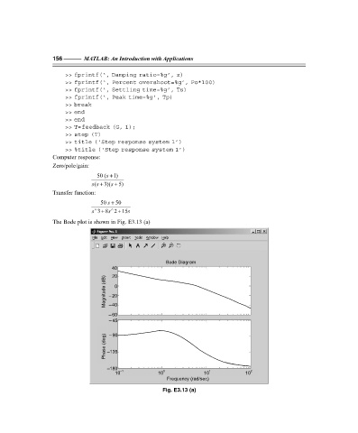
The Bode plot is shown in Fig. E3.13 (a)

Bode Diagram
40
(dB) 20 0
Magnitude –20

–40
–60
–45

(deg) –90

Phase –135

–180
10 –1 10 0 10 1 10 2
Frequency (rad/sec)
Fig. E3.13 (a)

F:\Final Book\Sanjay\IIIrd Printout\Dt. 10-03-09