Page 170 - MATLAB an introduction with applications

Control Systems ——— 155

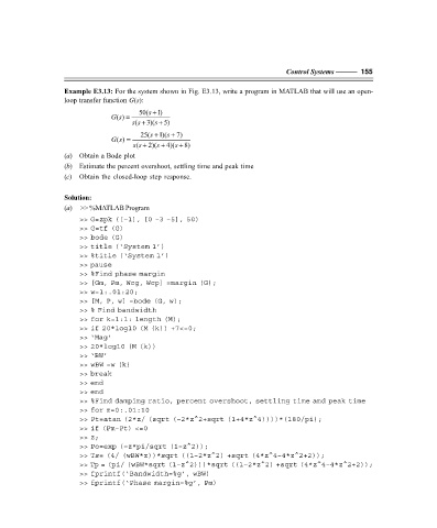
Example E3.13: For the system shown in Fig. E3.13, write a program in MATLAB that will use an open-
loop transfer function G(s):
50(s + 1)
() =
Gs
( ss + 3)(s + 5)
25(s + 1)(s + 7)
() =
Gs
( s s + 2)(s + 4)(s + 8)
(a) Obtain a Bode plot
(b) Estimate the percent overshoot, settling time and peak time
(c) Obtain the closed-loop step response.

Solution:
(a) >> %MATLAB Program
>> G=zpk ([–1], [0 –3 –5], 50)
>> G=tf (G)
>> bode (G)
>> title (‘System 1’)
>> %title (‘System 1’)
>> pause
>> %Find phase margin
>> [Gm, Pm, Wcg, Wcp] =margin (G);
>> w=1:.01:20;
>> [M, P, w] =bode (G, w);
>> % Find bandwidth
>> for k=1:1: length (M);
>> if 20*log10 (M (k)) +7<=0;
>> ‘Mag’
>> 20*log10 (M (k))
>> ‘BW’
>> wBW =w (k)
>> break
>> end
>> end
>> %Find damping ratio, percent overshoot, settling time and peak time
>> for z=0:.01:10
>> Pt=atan (2*z/ (sqrt (–2*z^2+sqrt (1+4*z^4))))*(180/pi);
>> if (Pm–Pt) <=0
>> z;
>> Po=exp (–z*pi/sqrt (1–z^2));
>> Ts= (4/ (wBW*z))*sqrt ((1–2*z^2) +sqrt (4*z^4–4*z^2+2));
>> Tp = (pi/ (wBW*sqrt (1–z^2)))*sqrt ((1–2*z^2) +sqrt (4*z^4–4*z^2+2));
>> fprintf(‘Bandwidth=%g’, wBW)
>> fprintf(‘Phase margin=%g’, Pm)

F:\Final Book\Sanjay\IIIrd Printout\Dt. 10-03-09