Page 168 - MATLAB an introduction with applications

Control Systems ——— 153

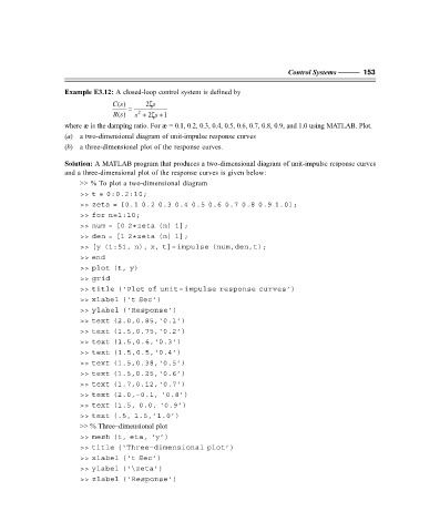
Example E3.12: A closed-loop control system is defined by
ζ
Cs = 2 s
()
2
Rs s +ζ 1
2 s +
()
where æ is the damping ratio. For æ = 0.1, 0.2, 0.3, 0.4, 0.5, 0.6, 0.7, 0.8, 0.9, and 1.0 using MATLAB. Plot.
(a) a two-dimensional diagram of unit-impulse response curves
(b) a three-dimensional plot of the response curves.
Solution: A MATLAB program that produces a two-dimensional diagram of unit-impulse response curves
and a three-dimensional plot of the response curves is given below:
>> % To plot a two-dimensional diagram
>> t = 0:0.2:10;
>> zeta = [0.1 0.2 0.3 0.4 0.5 0.6 0.7 0.8 0.9 1.0];
>> for n=1:10;
>> num = [0 2*zeta (n) 1];
>> den = [1 2*zeta (n) 1];
>> [y (1:51, n), x, t]= impulse (num,den,t);
>> end
>> plot (t, y)
>> grid
>> title (‘Plot of unit– impulse response curves’)
>> xlabel (‘t Sec’)
>> ylabel (‘Response’)
>> text (2.0,0.85,‘0.1’)
>> text (1.5,0.75,‘0.2’)
>> text (1.5,0.6,‘0.3’)
>> text (1.5,0.5,‘0.4’)
>> text (1.5,0.38,‘0.5’)
>> text (1.5,0.25,‘0.6’)
>> text (1.7,0.12,‘0.7’)
>> text (2.0,–0.1, ‘0.8’)
>> text (1.5, 0.0, ‘0.9’)
>> text (.5, 1.5,’1.0’)
>> % Three–dimensional plot

>> mesh (t, eta, ‘y’)
>> title (‘Three–dimensional plot’)
>> xlabel (‘t Sec’)
>> ylabel (‘\zeta’)
>> zlabel (‘Response’)

F:\Final Book\Sanjay\IIIrd Printout\Dt. 10-03-09