Page 175 - MATLAB an introduction with applications

160 ——— MATLAB: An Introduction with Applications

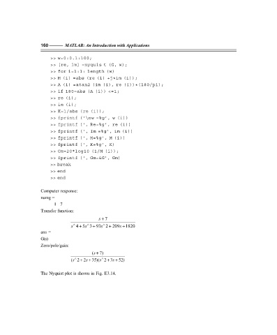
>> w=0:0.1:100;
>> [re, im] =nyquis t (G, w);
>> for i=1:1: length (w)
>> M (i) =abs (re (i) +j*im (i));
>> A (i) =atan2 (im (i), re (i))*(180/pi);
>> if 180–abs (A (i)) <=1;
>> re (i);
>> im (i);
>> K=1/abs (re (i));
>> fprintf (‘\nw =%g’, w (i))
>> fprintf (‘, Re=%g’, re (i))
>> fprintf (‘, Im =%g’, im (i))
>> fprintf (‘, M=%g’, M (i))
>> fprintf (‘, K=%g’, K)
>> Gm=20*log10 (1/M (i));
>> fprintf (‘, Gm=&G’, Gm)
>> break
>> end
>> end

Computer response:
numg =
1 7
Transfer function:
s + 7
+
s ∧ 4 5 3 93 2 209 +s ∧ + s ∧ + s 1820
ans =
G(s)
Zero/pole/gain:
( +s 7)
+
+
(s ∧ 2 2 +s 35)(s ∧ 2 3 +s 52)
The Nyquist plot is shown in Fig. E3.14.

F:\Final Book\Sanjay\IIIrd Printout\Dt. 10-03-09