Page 98 - MATLAB an introduction with applications

MATLAB Basics ——— 83

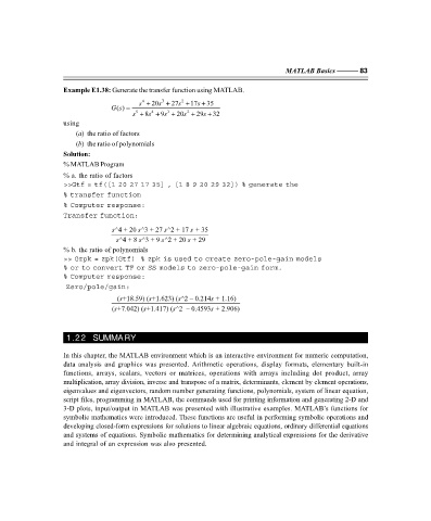
Example E1.38: Generate the transfer function using MATLAB.

s + 20s + 27s + 17s + 35
3
2
4
()Gs =
s + 8s + 9s + 20s + 29s + 32
3
4
5
2
using
(a) the ratio of factors
(b) the ratio of polynomials
Solution:
% MATLAB Program
% a. the ratio of factors
>>Gtf = tf([1 20 27 17 35] , [1 8 9 20 29 32]) % generate the
% transfer function
% Computer response:
Transfer function:
s ^4 + 20 ^3 + 27 ^2 + 17 + 35
s
s
s

s
^4 + 8 ^3 + 9 ^2 + 20 + 29
s
s
s
% b. the ratio of polynomials
>> Gzpk = zpk(Gtf) % zpk is used to create zero-pole-gain models
% or to convert TF or SS models to zero-pole-gain form.
% Computer response:
Zero/pole/gain:
s
s
s
( +18.59) ( +1.623) ( ^2 – 0.214 + 1.16)
s

s
s
( +7.042) ( +1.417) ( ^2 – 0.4593 + 2.906)
s
s
1.22 SUMMARY
In this chapter, the MATLAB environment which is an interactive environment for numeric computation,
data analysis and graphics was presented. Arithmetic operations, display formats, elementary built-in
functions, arrays, scalars, vectors or matrices, operations with arrays including dot product, array
multiplication, array division, inverse and transpose of a matrix, determinants, element by element operations,
eigenvalues and eigenvectors, random number generating functions, polynomials, system of linear equation,
script files, programming in MATLAB, the commands used for printing information and generating 2-D and
3-D plots, input/output in MATLAB was presented with illustrative examples. MATLAB’s functions for
symbolic mathematics were introduced. These functions are useful in performing symbolic operations and
developing closed-form expressions for solutions to linear algebraic equations, ordinary differential equations
and systems of equations. Symbolic mathematics for determining analytical expressions for the derivative
and integral of an expression was also presented.

F:\Final Book\Sanjay\IIIrd Printout\Dt. 10-03-09