Page 94 - MATLAB an introduction with applications

MATLAB Basics ——— 79

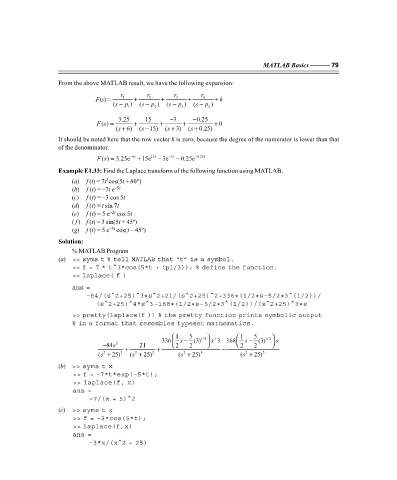
From the above MATLAB result, we have the following expansion:

r r r r
F(s) = 1 + 2 + 3 + 4 + k
(s − p ) (s − p ) (s − p ) (s − p )
1 2 3 4
3.25 15 − 3 − 0.25
() =
Fs + + + + 0
( + 6) ( − 15) ( + 3) ( + 0.25)
s
s
s
s
It should be noted here that the row vector k is zero, because the degree of the numerator is lower than that
of the denominator.
( ) =
Fs 3.25e − 6t + 15e 15t − 3e − 3t − 0.25e − 0.25t
Example E1.33: Find the Laplace transform of the following function using MATLAB.
3
(a) f (t) = 7t cos(5t + 60°)
(b) f (t) = –7t e –5t
(c) f (t) = –3 cos 5t
(d) f (t) = t sin 7t
–2t
(e) f (t) = 5 e cos 5t
( f ) f (t) = 3 sin(5t + 45º)
–3t
(g) f (t) = 5 e cos(t – 45º)
Solution:
% MATLAB Program
(a) >> syms t % tell MATLAB that “t” is a symbol.
>> f = 7 * t^3*cos(5*t + (pi/3)); % define the function.
>> laplace( f )
ans =
–84/(s^2+25)^3 * s^2+21/(s^2+25)^2+336 * (1/2 * s–5/2 * 3^(1/2))/
(s^2+25)^4*s^3–168*(1/2*s–5/2*3^(1/2))/(s^2+25)^3 *s
>> pretty(laplace(f )) % the pretty function prints symbolic output
% in a format that resembles typeset mathematics.
 1 5 1/ 2   1 5 1/ 2 
336  s − (3)  s ∧ 3 168  s − (3)  s
2
− 84s + 21 +  2 2  −  2 2 
2
2
(s + 25) 3 (s + 25) 2 (s + 25) 4 (s + 25) 3
2
2
(b) >> syms t x
>> f = –7*t*exp(–5*t);
>> laplace(f, x)
ans =
–7/(x + 5)^2
(c) >> syms t x
>> f = –3*cos(5*t);
>> laplace(f,x)
ans =
–3*x/(x^2 + 25)

F:\Final Book\Sanjay\IIIrd Printout\Dt. 10-03-09