Page 93 - MATLAB an introduction with applications

78 ——— MATLAB: An Introduction with Applications

r =
–1.3849 + 1.2313i
–1.3849 – 1.2313i
0.3849 – 0.4702i
0.3849 + 0.4702i
p =
–0.8554 + 3.0054i
–0.8554 – 3.0054i
–1.6446 + 1.3799i
–1.6446 – 1.3799i
k =
1
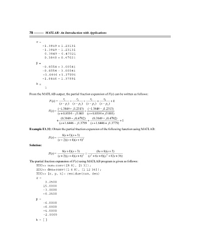
From the MATLAB output, the partial fraction expansion of F(s) can be written as follows:
r r r r
Fs 1 + 2 + 3 + 4 + k
() =
s
s
s
s
( − p 1 ) ( − p 2 ) ( − p 3 ) ( − p 4 )
−
( 1.3849+ j 1.2313) ( 1.3849 − j 1.2313)
−
F(s) = +
(s + 0.8554 − j 3.005 (s + 0.8554 + j 3.005)
(0.3849 − j 0.4702) (0.3849 + j 0.4702)
+ (s + 1.6446 − j 1.3799 + (s + 1.6446 + j 1.3779) + 1
Example E1.32: Obtain the partial fraction expansion of the following function using MATLAB:
8(s + 1)(s + 3)
F(s) =
(s + 2)(s + 4)(s + 6) 2
Solution:
8(s + 1)(s + 3) (8s + 8)(s + 3)
F(s) = =
2
(s + 2)(s + 4)(s + 6) 2 (s + 6s + 8)(s + 12s + 36)
2
The partial fraction expansion of F(s) using MATLAB program is given as follows:
EDU>> num=conv([8 8], [1 3]);
EDU>> den=conv([1 6 8], [1 12 36]);
EDU>> [r, p, k]= residue(num, den)
r =
3.2500
15.0000
–3.0000
–0.2500
p =
–6.0000
–6.0000
–4.0000
–2.0000
k = [ ]

F:\Final Book\Sanjay\IIIrd Printout\Dt. 10-03-09