Page 92 - MATLAB an introduction with applications

MATLAB Basics ——— 77

r =
–0.5357 – 1.0394i
–0.5357 + 1.0394i
0.5357 – 0.1856i
0.5357 + 0.1856i
p =
–1.5000 + 1.3229i
–1.5000 – 1.3229i
–0.0000 + 1.7321i
–0.0000 – 1.7321i
k = [ ]
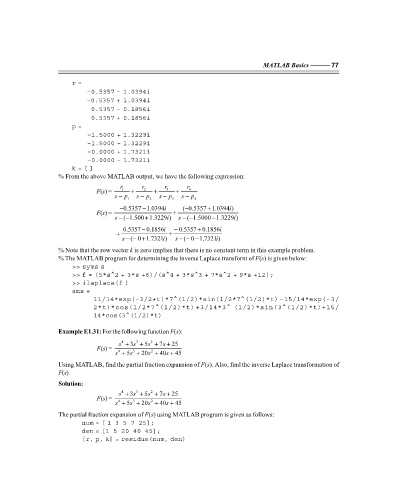
% From the above MATLAB output, we have the following expression:
r r r r
F(s) = 1 + 2 + 3 + 4
s − p 1 s − p 2 s − p 3 s − p 4
+
− 0.5357 1.0394i ( 0.5357 1.0394 )
−
−
i
F(s) = +
−
−
i
( 1.500 1.3229 )
s −− + i s − ( 1.5000 1.3229 )
+
−
0.5357 0.1856i − 0.5357 0.1856i
+ +
s −− + s −− −
( 0 1.7321 ) i
( 0 1.7321 ) i
% Note that the row vector k is zero implies that there is no constant term in this example problem.
% The MATLAB program for determining the inverse Laplace transform of F(s) is given below:
>> syms s
>> f = (5*s^2 + 3*s +6)/(s^4 + 3*s^3 + 7*s^2 + 9*s +12);
>> ilaplace(f )
ans =
11/14*exp(–3/2 * t)*7^(1/2)*sin(1/2*7^(1/2)*t) –15/14*exp(–3/
2*t)*cos(1/2*7^(1/2)*t) +3/14*3^ (1/2)*sin(3^(1/2)*t)+15/
14*cos(3^(1/2)*t)
Example E1.31: For the following function F(s):
3
s
s
s 4 + 3 + 5s 2 + 7 + 25
F(s) =
s 4 + 5s 3 + 20s 2 + 40 + 45
s
Using MATLAB, find the partial fraction expansion of F(s). Also, find the inverse Laplace transformation of
F(s).
Solution:
3
s
s 4 + 3 + 5s 2 + 7 + 25
s
F(s) =
s
s 4 + 5s 3 + 20s 2 + 40 + 45
The partial fraction expansion of F(s) using MATLAB program is given as follows:
num = [ 1 3 5 7 25];
den = [1 5 20 40 45];
[r, p, k] = residue(num, den)

F:\Final Book\Sanjay\IIIrd Printout\Dt. 10-03-09