Page 97 - MATLAB an introduction with applications

82 ——— MATLAB: An Introduction with Applications

Solution:
% MATLAB Program
>> syms s % tell MATLAB that “s” is a symbol.
>>G = (s^2 + 9*s +7)*(s + 7)/[(s + 2)*(s + 3)*(s^2 + 12*s + 150)]; % define
the function.
>>pretty(G) % the pretty function prints symbolic output
% in a format that resembles typeset mathematics.
( + 9 + 7)( + 7)
s
s
s
( + 2)( + 3)( + 12 + 150)
s
s
s
s
>> g = ilaplace(G); % inverse Laplace transform
>>pretty(g)
44 2915
−
−
−
− 7/ 26exp( 2 ) + exp( 3 ) + exp( 6 )cos(114 )
½
t
t
t
t
123 3198
889
1/ 2
−
+ exp( 6 )114 1/ 2 sin(114 t )
t
20254
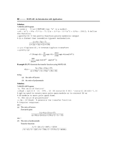
Example E1.37: Generate the transfer function using MATLAB.
3(s + 9)(s + 21)(s + 57)
() =
Gs
2
2
( ss + 30)(s + 5s + 35)(s + 28s + 42)
using
(a) the ratio of factors
(b) the ratio of polynomials
Solution:
% MATLAB Program
‘a. The ratio of factors’
>>Gzpk = zpk([–9 –21 –57] , [0 –30 roots([1 5 35]) 'roots([1 28 42])'],3)
% zpk is used to create zero-pole-gain models or to convert TF or
% SS models to zero-pole-gain form.
‘b. The ratio of polynomials’
>> Gp = tf(Gzpk) % generate the transfer function
% Computer response:
ans =
(a) The ratio of factors
Zero/pole/gain:
3 ( +9) ( +21) ( +57)
s
s
s
( +30) ( +26.41) ( +1.59) ( ^2 + 5 + 35)
ss s s s s
ans =
(b) The ratio of polynomials
Transfer function:
s
3 ^3 + 261 ^2 + 5697 + 32319
s
s

s
s
s
s
s ^6 + 63 ^5 + 1207 ^4 + 7700 ^3 + 37170 ^2 + 44100 s
F:\Final Book\Sanjay\IIIrd Printout\Dt. 10-03-09