Page 121 - MATLAB Recipes for Earth Sciences

114 5 Time-Series Analysis

0

5

10

15

20
Time 25

30
1.0
35

40 0.5

45

0.0
0 5 10 15 20 25 30 35 40 45 50
Time
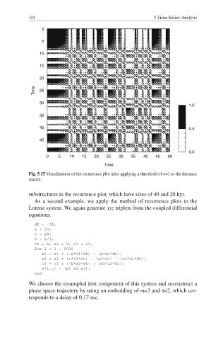
Fig. 5.15 Visualization of the recurrence plot after applying a threshold of ε=1 to the distance
matrix.

substructures in the recurrence plot, which have sizes of 40 and 20 kyr.
As a second example, we apply the method of recurrence plots to the
Lorenz system. We again generate xyz triplets from the coupled differential
equations.

dt = .01;
s = 10;
r = 28;
b = 8/3;
x1 = 8; x2 = 9; x3 = 25;
for i = 1 : 5000
x1 = x1 + (-s*x1*dt) + (s*x2*dt);
x2 = x2 + (r*x1*dt) - (x2*dt) - (x3*x1*dt);
x3 = x3 + (-b*x3*dt) + (x1*x2*dt);
x(i,:) = [x1 x2 x3];
end
We choose the resampled first component of this system and reconstruct a

phase space trajectory by using an embedding of m=3 and τ=2, which cor-
responds to a delay of 0.17 sec.