Page 117 - MATLAB Recipes for Earth Sciences

110 5 Time-Series Analysis

t = 0.01 : 0.01 : 50;
plot(t, x(:,1))
xlabel('Time')
ylabel('Temperature')

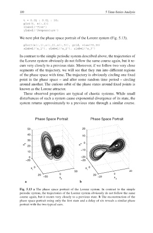
We next plot the phase space portrait of the Lorenz system (Fig. 5.13).

plot3(x(:,1),x(:,2),x(:,3)), grid, view(70,30)
xlabel('x_1'), ylabel('x_2'), zlabel('x_3')

In contrast to the simple periodic system described above, the trajectories of
the Lorenz system obviously do not follow the same course again, but it re-
curs very closely to a previous state. Moreover, if we follow two very close
segments of the trajectory, we will see that they run into different regions
of the phase space with time. The trajectory is obviously circling one fi xed
point in the phase space – and after some random time period – circling
around another. The curious orbit of the phase states around fi xed points is
known as the Lorenz attractor.
These observed properties are typical of chaotic systems. While small
disturbances of such a system cause exponential divergence of its state, the
system returns approximately to a previous state through a similar course.

Phase Space Portrait Phase Space Portrait

50 20
40
10
30
0
3
x x 3
20
−10
10
0 −20
−20 −20
x 0 x 0
1 1
50 20
20 0 20 0
−50 x −20 x
2 2
a b
Fig. 5.13 a The phase space portrait of the Lorenz system. In contrast to the simple
periodic system, the trajectories of the Lorenz system obviously do not follow the same
course again, but it recurs very closely to a previous state. b The reconstruction of the

phase space portrait using only the first state and a delay of six reveals a similar phase
portrait with the two typical ears.