Page 114 - MATLAB Recipes for Earth Sciences

5.6 Nonlinear Time-Series Analysis (by N. Marwan) 107

systems. The method is now a widely accepted tool for the nonlinear analy-
sis of short and nonstationary data sets.

Phase Space Portrait

The starting point of most nonlinear data analysis is the construction of the
phase space portrait of a system. The state of a system can be described by
its state variables x (t), x (t), …, x (t). As example, suppose the two variables
1 2 d
temperature and pressure to describe the thermodynamic state of the Earth·s
mantle as a complex system. The d state variables at time t form a vector
in a d-dimensional space, the so-called phase space. The state of a system
typically changes in time. The vector in the phase space therefore describes
a trajectory representing the temporal evolution, i.e., the dynamics of the
system. The course of the trajectory provides all important information on
the dynamics of the system, such as periodic or chaotic systems having char-
acteristic phase space portraits.
In many applications, the observation of a natural process does not yield
all possible state variables, either because they are not known or they cannot
be measured. However, due to coupling between the system·s components,
we can reconstruct a phase space trajectory from a single observation u :
i

where m is the embedding dimension and τ is the time delay (index based;
the real time delay is τ = ¨t). This reconstruction of the phase space is called
time delay embedding. The phase space reconstruction is not exactly the
same to the original phase space, but its topological properties are pre-
served, if the embedding dimension is large enough. In practice, the embed-
ding dimension has to be larger then twice the phase space dimension, or

exactly m>2d+1. The reconstructed trajectory is sufficient enough for the
subsequent data analysis.
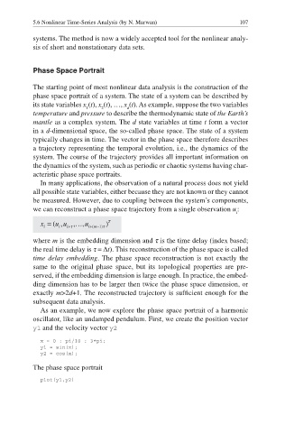
As an example, we now explore the phase space portrait of a harmonic
oscillator, like an undamped pendulum. First, we create the position vector
y1 and the velocity vector y2
x = 0 : pi/10 : 3*pi;
y1 = sin(x);
y2 = cos(x);
The phase space portrait

plot(y1,y2)