Page 111 - MATLAB Recipes for Earth Sciences

104 5 Time-Series Analysis

Interpolated Signals
15
10 Linearly-interpolated
data series
5
0
y(t) −5
Original data point
−10
−15 Spline-interpolated
data series
−20
−25
350 360 370 380 390 400 410 420 430 440 450
t
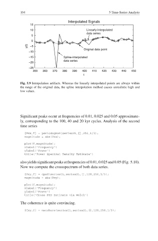
Fig. 5.9 Interpolation artifacts. Whereas the linearly interpolated points are always within
the range of the original data, the spline interpolation method causes unrealistic high and
low values.

Significant peaks occur at frequencies of 0.01, 0.025 and 0.05 approximate-

ly, corresponding to the 100, 40 and 20 kyr cycles. Analysis of the second
time series

[Pxx,f] = periodogram(series2L,[],256,1/3);
magnitude = abs(Pxx);
plot(f,magnitude);
xlabel('Frequency')
ylabel('Power')
title('Power Spectral Density Estimate')

also yields significant peaks at frequencies of 0.01, 0.025 and 0.05 (Fig. 5.10).

Now we compute the crossspectrum of both data series.
[Pxy,f] = cpsd(series1L,series2L,[],128,256,1/3);
magnitude = abs(Pxy);

plot(f,magnitude);
xlabel('Frequency')
ylabel('Power')
title('Cross PSD Estimate via Welch')

The coherence is quite convincing.
[Cxy,f] = mscohere(series1L,series2L,[],128,256,1/3);