Page 116 - MATLAB Recipes for Earth Sciences

5.6 Nonlinear Time-Series Analysis (by N. Marwan) 109

Integrating the differential equation yields a simple MATLAB code for
computing the xyz triplets of the Lorenz attractor. As system parameters
controlling the chaotic behaviour we use s=10, r=28 and b=8/3, the time
delay is dt=0.01. The initial values are x1=6, x2=9 and x3=25, that can
certainly be changed at other values.

dt = .01;
s = 10;
r = 28;
b = 8/3;
x1 = 8; x2 = 9; x3 = 25;
for i = 1 : 5000
x1 = x1 + (-s*x1*dt) + (s*x2*dt);
x2 = x2 + (r*x1*dt) - (x2*dt) - (x3*x1*dt);
x3 = x3 + (-b*x3*dt) + (x1*x2*dt);
x(i,:) = [x1 x2 x3];
end

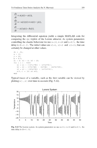
Typical traces of a variable, such as the first variable can be viewed by
plotting x(:,1) over time in seconds (Fig. 5.12).

Lorenz System
20
15
Temperature 10
5
0
−5
−10
−15
−20
0 5 10 15 20 25 30 35 40 45 50
Time

Fig. 5.12 The Lorenz system. As system parameters we use s=10, r=28 and b=8/3, the
time delay is dt=0.01.